Can a learned rule tell a fluid code what the ions are doing?
Do the learned corrections produce useful forces?
Fine-tuned force MSE falls by 62% in the training regime and 42% in an unseen run, relative to omitting anisotropic stress. Disagreement also beats random region selection.
Watch the physical movies → · Explore the measured results →
Shared pretraining, different closure objectives
Pretrained codec
- learns from
- 5 particle runs, all 10 fields
- job
- some fields are hidden; rebuild all of them. Half the time the hidden ones are the two temperatures.
- good for
- compressing supplied plasma states, and inferring hidden temperatures; this is not yet an autonomous emulator
Our network
- learns from
- the same 5 runs, from scratch
- job
- only one: given density, flow, field and temperature, predict how much hotter the ions are across the field than along it
- good for
- the closure alone; never saw pretraining
Fine-tuned complete
- learns from
- the codec's encoder, then the same 5 runs
- job
- our network's job, starting from what the codec already knows
- good for
- testing whether pretraining helps the closure
The training-run view uses held-out times; the larger-box and real-proton-mass runs are excluded from training. Post-trained codec and fine-tuned closure head are distinct model variants.
The codec reconstructs held-out simulation frames
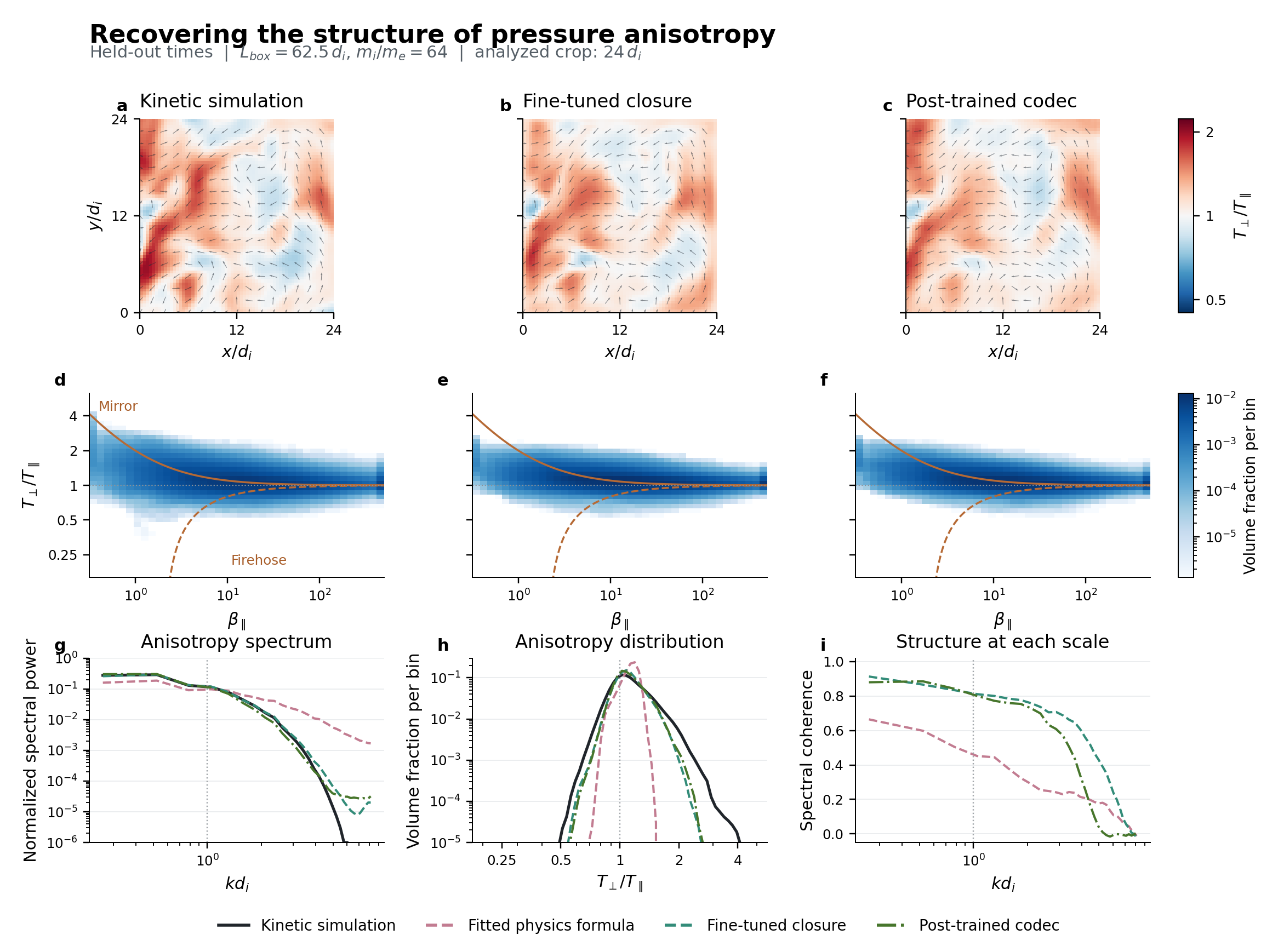
A slice through the middle of one chunk, over 20 snapshots the networks never trained on. Left: the particle simulation. Middle: the codec's rebuild from its compressed copy. Right: the difference, five times magnified. "Error" is the typical difference from the simulation as a share of the field's natural variation, over the whole 3D chunk: 0% is perfect, a flat guess scores about 100%. "Small-scale fluctuations" removes each field's 2 di running mean and keeps only the structure near the ion scale, the hard part to rebuild.
Where the ions run hotter across or along the magnetic field
Arrows show the magnetic field direction. MHD paints everything white. Pinned, Braginskii and the physics formula are the classic closures from the literature, with their numbers fitted to our training runs. "Error" as above: MHD sits near 100%, lower is better. The codec and our network only see density, flow, field and temperature, never the true colours. The run, play and time controls above drive this movie too.
Does the rebuilt plasma have the right physics?
"Power at each scale" shows how much structure there is at each size; matching curves mean similar spectral shape. Each spectrum is normalized separately, so this does not establish equal total power. "How well each scale is reproduced" is the coherence between simulation and prediction at each size: 1 means perfectly correlated structure at that scale (amplitude can still differ), 0 means uncorrelated. Pick "temperature imbalance" to compare the closures scale by scale.
How often each amount of imbalance occurs. MHD puts everything on the dashed line. In the simulation, about a third of the volume is more than 25% off it; that is where MHD is wrong and the closures add the missing force. Learned models still miss part of the tails near and beyond the diagnostic instability thresholds.
x: parallel plasma β (thermal over magnetic pressure). y: T⊥/T∥. Both log scales. This is the textbook diagram for kinetic plasmas. Above the solid line the plasma is mirror-unstable; below the dashed line, firehose-unstable. A good closure puts the right amount of plasma near those limits.
Below and above the ion skin depth
"Raw" is the particle simulation at full resolution, down to its 3-electron-skin-depth output grid. The other settings coarse-grain it to 1, 2, 4 or 8 ion skin depths, like the grid of a fluid code. At each scale the classic closures are refit and a closure network is trained from scratch; the pretrained codec exists only at 1 di. Errors are over 20 snapshots the models never saw: 0% perfect, a flat guess about 100%.
x: the coarse-graining scale, how coarse the fluid code's grid is. y: closure error at that scale, lower is better. MHD is the dashed line. Scales larger than a third of the chunk are left out, since almost no structure survives there. The 2 and 4 di trainings are complete; matched-crop maps are not yet synchronized into this chart. Their separate evaluation summaries appear below. Missing curves do not mean zero performance.
The full spectrum of the raw simulation, from the box down to the grid. Each dashed line marks where a coarse-graining scale cuts off structure: everything to its right is what a fluid code at that resolution cannot see and a closure must stand in for.
MHD assumes ion pressure is the same in every direction. It isn't.
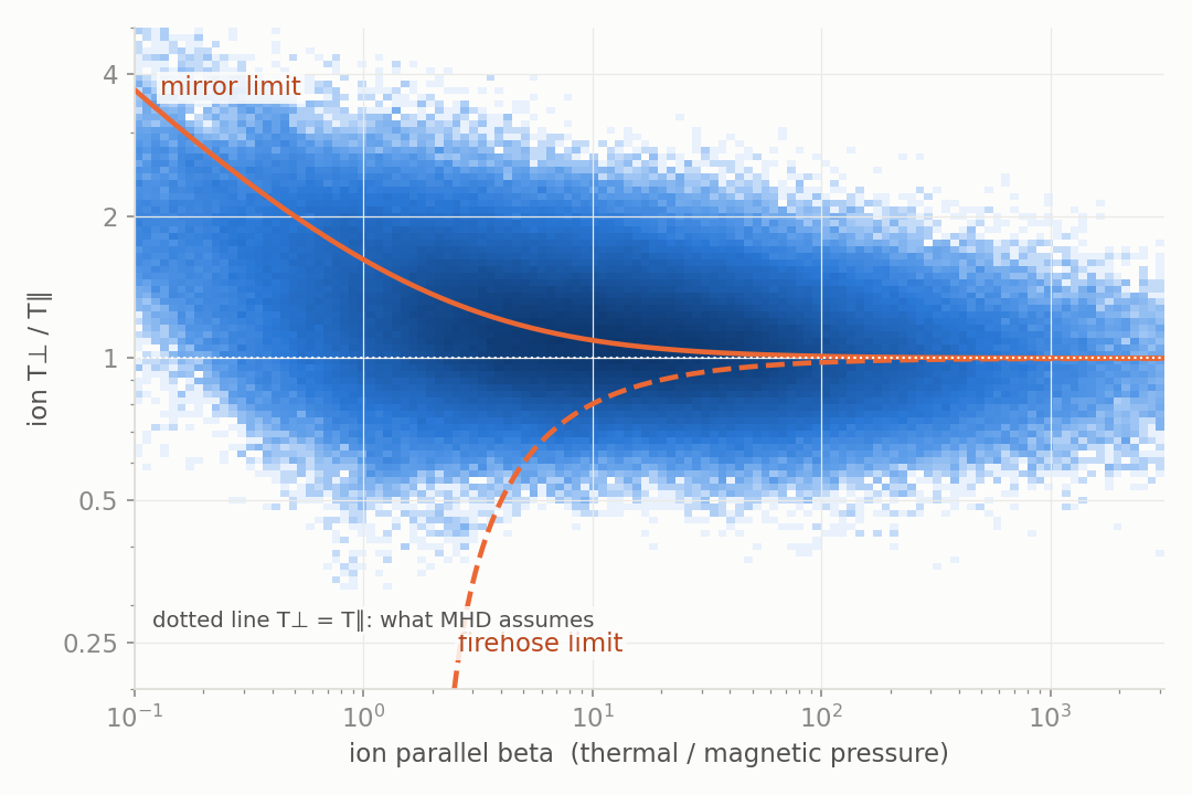
Each dot is a place in a particle simulation. MHD assumes every dot sits on the dotted line at 1.
Two steps: learn the plasma, then learn the missing force
The first try learned nothing. The fixed one rebuilds almost everything.
Reconstruction error, lower is better, log scale. The tiles show how much of each field the fixed codec rebuilds on runs it trained on.
Who predicts the missing force best?
Score: 1 is perfect, 0 is guessing the average. Bars stop at −1; hover for the real value. fine-tuning complete
Hide the magnetic field or the flow and the closure collapses
The ablation is consistent with a role for field-aligned flow and strain. In this ablation, magnetic field and flow are the most informative inputs; this does not establish that other quantities are physically irrelevant.
Earlier scratch-network sweep at fixed box size
Historical scratch-network comparison, not the latest pretrained result. Each line fixes box size; bars show snapshot spread. The pretrained model retains R² = 0.46 at mass ratio 1836 in the 23.3 d_i box.
The current MHD and kinetic baselines differ at large scales
Share of magnetic energy at the largest scales. These runs are not a controlled closure intervention: mass ratio, beta, forcing and numerical dissipation can also differ.
From learned kinetic physics to evolving fluid simulations
Can a representation learned from expensive simulations improve a cheaper model during evolution, and identify when that model needs higher-fidelity information? The kinetic results here establish offline reconstruction and anisotropy inference. The next decisive test is optimization inside an evolving fluid solver.
The TCV foundation-model work supplies the fusion counterpart: transferable representations in realistic edge geometry, followed by corrections between matched simulation fidelities. Offline routing is a first test of reliability; live conservative kinetic-patch coupling remains a longer-term aim.
Newly completed evaluations
2 dᵢ and 4 dᵢ closure training and raw-field pretraining are complete. The 8 dᵢ closure job was still running when this page was assembled. This is a dated snapshot, not live monitoring.
| Filter / model | Held-out times | 125 dᵢ, mass 16 | 125 dᵢ, mass 64 | 23.3 dᵢ, mass 1836 |
|---|---|---|---|---|
| 2 dᵢ, scratch | 0.539 | 0.383 | 0.296 | -0.549 |
| 4 dᵢ, scratch | 0.332 | 0.239 | 0.242 | -2.217 |
These independently trained coarse-scale models retain some large-box skill but fail on the real-mass case. Compare them only within their evaluation protocol; they are not the codec models in the physics movies above.
Raw-field pretraining reconstructs fluctuations with mean field R² of 0.951 on held-out times, 0.957 in the larger box, and 0.940 at real proton mass ratio. These are supplied-frame reconstruction scores, not future prediction or corrected fluid evolution.
Physics figures for discussion
Held-out-time figure (PDF) · Unseen-box figure (PDF)