Every result here is from one simulated trajectory, several models are under-trained, and the gate suite is small and still evolving. Numbers are approximate and, where two computations disagree (e.g. a mid-plane slice vs a full-volume evaluation), we say so. Treat comparisons as directional signal about where to look next, not as benchmark rankings.
1The enemy: the freeze
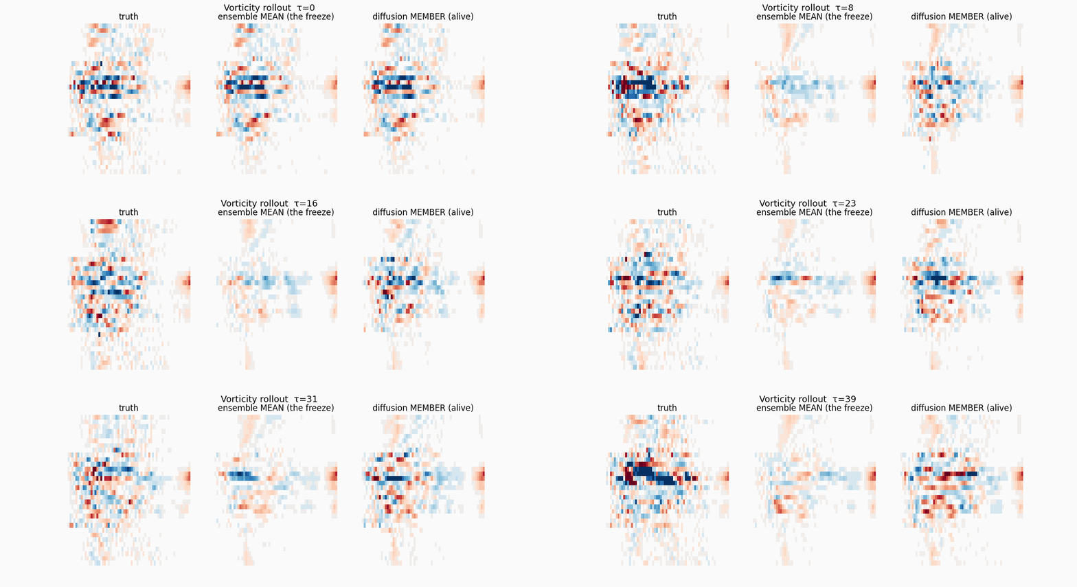
Turbulence is chaotic: from one state many futures are equally consistent, and a model trained on pointwise error is forced to output their average. The average of many decorrelated eddies is smooth — so the model keeps the large-scale predictable fields and deletes the small-scale turbulence. We call this the freeze.
It is not a bug to be tuned away; it is the optimum of the wrong objective. With Gap = E[Var(Y|X)]/Var(Y) defined per scale (per Fourier mode), the MSE-optimal prediction is the conditional mean E[Y|X], whose variance at that scale → 0 as Gap → 1 — and chaotic predictability decays fastest at small scales, hence the high-k collapse (the conditional-uncertainty-gap argument of Green et al. 2026, arXiv:2606.04342, applied here per Fourier mode; the effect itself is classical — ensemble-mean damping, Leith 1974). For τ ≫ τcorr the FreezeRatio below tends to the climatological variance ratio σpred/σtruth — a variance check, not a skill score. We measure the freeze with the
A working rule we adopted follows from this: we try not to select a model or lead with a headline on validation MSE, since that is the metric the freeze minimizes. We lean instead on FreezeRatio, spectral fidelity, transport statistics, and ensemble calibration. This is a heuristic, not a theorem, and each of those diagnostics has its own failure modes (noted where relevant).
2Data: one trajectory
All models train on a Hermes-3 / BOUT++ simulation of TCV — shot 85604 for train/validation, shot 85606 held out as test. Channel sets range from four to twelve fields across the ablations; the physics-correct final set is the five independent evolved fields (n, Te, Ti, φ, V∥), with derived vorticity ω on the earlier sets. All on the native flux-aligned grid 64×32×81 (radial × poloidal × toroidal; toroidal Fourier-resampled to 88 for the patch models), one-fifth-torus wedge (zperiod=5), boundaries wall / wall / periodic. The record is one long time series. The correlation time is field-dependent: median τcorr ranges from about 1 frame for vorticity to ~11 frames for the potential (§7). So the step dt=1 is well inside τcorr for the smooth fields but is comparable to it for vorticity — which is one reason pointwise vorticity error becomes meaningless quickly. The single-trajectory constraint is the data-efficiency bet: a method that needs thousands of shots is unlikely to transfer to a new machine.

3The gate suite (how every model is scored)
The fields split into predictable and turbulent. Density is smooth and large-scale (models reach Pearson R ≈ 0.99); vorticity is thin, flux-surface-aligned filaments that break first. That contrast is much of the problem here.
Every model is scored on the same gates: FreezeRatio(τ) per field; spectral fidelity (binned high-k NMSE); VRMSE (>1 = worse than the time-mean); radial E×B flux Γr = ⟨n vr⟩ (profile correlation, and its intermittent PDF / kurtosis); and, for ensembles, spread-skill (calibration ≈ 1) resolved per wavenumber. The flux is an index-space proxy: we take vr ≈ −∂φ/∂y with metric factors (hθ, B(R) variation) omitted and weighted identically for truth and model, so relative and PDF-shape comparisons are meaningful but absolute magnitudes are not. The convention assumes the Hermes-3 dumps are in shifted-metric (z = toroidal angle) coordinates.
4ViT3D: the deterministic baseline, and where it froze
We started with a from-scratch deterministic operator. We tried more capacity, different time-strides, and augmentation; vorticity stayed in the frozen band throughout. That is the strongest hint in this notebook that the freeze is structural rather than a training deficiency — though an untried recipe could still prove us wrong.
Configuration. tcv_vit, a Walrus-style operator: strided-conv patch
tokenizer → full spatial attention + causal temporal attention → un-patchify. 44.8 M
parameters (hidden 256, projection 96, 6 blocks, 8 heads), 6-frame history,
predicting the RMS-normalized one-step increment under a pooled L1 loss, up to 400 epochs.
The toroidal axis is Fourier-resampled 81→88 (Gate-1a) so the patch grid divides evenly.
What we ran. A nine-run sweep over channel count (c4/c8/c12), toroidal jitter augmentation on/off, learning rate ((0.001, 0.0003, 0.0001)), and model size. The easy fields solve early (n/Te/φ: Pearson R ≈ 0.99, VRMSE ≈ 0.15 converged); vorticity pins at FreezeRatio ≈ 0.20, VRMSE ≥ 1, flat the entire run. (A logging bug initially truncated the metric curves to the early epochs; once fixed, the honest freeze curve is flat, 0.16→0.19 across 400 epochs.) A per-region failure atlas localized the missing motion to the X-point and divertor legs — exactly the high-shear, thin-filament regions. For context, capacity alone does not appear to be the cure even at scale: the Walrus paper's own 1.3 B pretrained operator reports median VRMSE 1.23 on its 3D MHD plasma benchmark (their evaluation, not ours — we did not finetune it on TCV).
The clean control. A variable-dt run (time-stride 1, 1–3, 1–5) forces the model to learn progressively harder big-increment tasks — and it demonstrably does: the pooled training loss converges to progressively higher plateaus (≈22 / 27 / 28 on its scaled axis). Vorticity FreezeRatio stays 0.22 / 0.21 / 0.18 (converged-window means): frozen at every stride. So, in these runs, the freeze does not look like under-training or a mismatched timescale.

The freeze shows up physically: the predicted radial flux keeps the right shape (profile correlation 0.89–0.99, since transport is governed by n and φ) but its net magnitude decays toward zero over the rollout while the truth sustains it. The arrow points at the architecture: plausibly a patch-conv tokenizer that low-passes high-k, together with a pooled point-wise loss. The later models are each a different attempt to work around one or both.
5GAOT / MAGNO: geometry overfit, but the objective moved the needle
GAOT was chosen for a specific reason: the published version carries three ingredients that, on paper, should each fight the freeze — a geometry-aware MAGNO encoder that respects the real flux-aligned grid, two z-scored time-to-target features, and a z-scored target derivative. We integrated all three carefully, and the result reframed the whole problem.
Configuration. MAGNO node→token graph → ViT → MAGNO decoder,
25 M parameters, flattening the grid into a physical
(R, Z, arc) point cloud — 64×32×44 = 90,112 nodes,
the same data as ViT3D with the toroidal axis coarsened by 2 (88→44) to fit the graph in memory. The ViT embedding dimension must be
divisible by 6 (coordinate dimension 3, lifting 48): 384 works, 512 does not.
Integration, with known-answer gates. We staged it so each layer was proven before the next. S1: a Cartesian torus-in-a-cube adapter (6/6 unit tests). S2: the freeze-fixes behind analytic known-answer tests — a drifting-sine field must give FreezeRatio 1 (moving) vs 0 (frozen) and a clean spectrum spike (4/4). S4: full-3D smoke green.
Wall 1 — geometry. The Cartesian embedding wasted 40% of latent tokens on empty cells (the torus doesn't fill a cube). Switching to a native cylinder embedding with balanced axes ([0.51, 0.99, 1.02] m) cut dead tokens to 13%. Wall 2 — memory. The node→token edge tensor is ~70× larger than a 2D graph: ~47 GB at batch 64 → OOM; only batch 8 fits (~72 GB).
A dead end we chased down. The z-scored target derivative has low variance (≈0.09), which looked like it might starve the loss. Rescaling it (variance 0.09→0.74) broke training outright — the loss pinned at exactly 1.000. Reverting to the stock normalization trained fine (prior runs had already fit to train MSE 0.043). The der-std "bug" was a non-problem: GAOT's failure is weak generalization, not weak fitting. (An earlier note blaming a der-std bug is superseded by this result.)
The generalization verdict, and the signal. On one trajectory GAOT overfits — train MSE descends to 0.043 while validation plateaus at the predict-zero floor (~0.096, train/val gap 0.006→0.017) over only ~55 independent states. But the same run — trained with the multi-horizon / all-to-all objective (job 6504528, cancelled at epoch 30) — showed vorticity climbing off the floor: FreezeRatio(τ=12) = 0.030 → 0.108 → 0.078 at epochs 10/20/30, noisy and non-monotonic, with the horizon-collapse flattening.
The tentative lesson we carried forward: it looks like the multi-step / all-to-all objective, more than the geometry, is what starts to move vorticity off the floor, while validation MSE stayed flat the whole time. We read this as a reason to keep the objective and set the geometry backbone aside — on the strength of one cancelled, under-trained run, so it is a lead to test, not a conclusion.
6JEPA / VICReg: a predictive latent discards what we need
The hypothesis was appealing: a predictive self-supervised encoder with a hard variance floor should make the collapsed (frozen) solution illegal, giving an anti-freeze latent that a diffusion model could then generate in. We ported it faithfully; it does prevent collapse, but seemingly the wrong kind. We found this one of the more clarifying negative results in these notes.
Configuration. The published Polymathic encoder runs Conv3d over (T, H, W) of a 2D field and squeezes the time axis — "its 3D is really 2D+time." We built a genuine 3D-spatial port: a per-frame ConvNeXt encoder (dims 16/32/64/128, residual blocks 3/3/9/3, three stride-2 downsamples, no time-collapse), temporal mean-pool to a block representation, then a 3D ConvPredictor maps context→target. Grid 64×32×88 → 8×4×11 (the same spatial grid as the LOLA latent; 128 latent channels here vs LOLA's 64). VICReg weights sim 2 / std 40 / cov 2: the variance floor (μ=40) is 20× the invariance term, so the encoder is trained primarily not to collapse and only secondarily to predict.
Health check. It works as advertised — 100% of latent dims stay active, latent FreezeRatio 1.60: no dimensional or temporal collapse. But "not collapsed" is not "keeps the turbulence." A held-out high-k probe (512 frames) exposes a monotonic predictability gradient.

A cleaner control. To rule out "the high-k is there but the probe can't read it," we trained an identical fresh voxel-shuffle decoder on each frozen latent — the only variable is the latent content — with a 15% validation split and early stopping so an over-trained decoder can't hallucinate small scales. It recovers the vorticity cascade to k≈0.50 (FreezeRatio 0.76) from the reconstructive AE latent, but only to k≈0.28 (FreezeRatio 0.68) from the predictive JEPA latent — ~2× less high-k. Crucially, bolting a reconstruction head directly onto the JEPA latent recovered nothing (break-k 0.26): the discarded high-k is gone from the latent, not merely un-decoded.

One more lever, ruled out. We also ran the VISReg variant (decoupled scale + Sliced-Wasserstein shape regularizer, with a Gaussian / Laplace / none shape knob) as a controlled swap on c4 and c5. Negative result: VICReg's covariance decorrelation term retains ~2× more high-k than VISReg — decorrelation, not the shape prior, seemed to be the active ingredient, and it was not enough. And because the edge turbulence is strongly non-Gaussian (TCV probe measurements report radial-flux-PDF flatness F = 107 against 3 for a Gaussian — Theodorsen et al. 2016; see also Garcia et al. 2007 — and our own simulation flux PDF is of the same order, §7), a Gaussian-in-latent generative step would likely re-freeze through the back door.
A tentative way to read it: predictive sufficiency need not be full-state sufficiency. JEPA seems to learn a predictive sufficient statistic and discard the rest, which could be useful for estimating a global plasma quantity from few shots but unhelpful for sampling the full turbulent state. If that reading holds, generation would want a reconstructive latent that keeps everything, which is the direction LOLA takes.
7LOLA: latent diffusion, the arm that stayed alive
The family that worked best in our tests: a reconstruction-trained autoencoder (keeps everything, per §6) with a diffusion model generating dynamics in its latent. The idea is that sampling the conditional distribution, rather than reporting its mean, is what lets small scales survive; our runs are consistent with that but are preliminary and from one trajectory. Getting here took a careful recipe extraction and a compression sweep before any dynamics model was trained.
Recipe extraction — code ≠ paper. Four passes over the released LOLA codebase found three shipped-vs-published divergences, each followed to the code: the AE loss is variance-normalized MSE in code but L1 in the paper (we used L1); the denoiser is azula EDM variance-exploding, not rectified flow; the optimizer is PSGD-Kron at lr 1e-5 (the README's real command, not the config default). This mattered: a hand-rolled AdamW overfit gate diverged (vmse 1.17→1.5e7), apparently because Adam's inverse-RMS-gradient step amplifies the deliberately-tiny identity-init gradients, while PSGD-Kron drove the same gate to ~1e-3. We reproduced the paper's AE table before going further.
M1 — the AE does not freeze. Fixing f8 spatial compression, we swept latent channels (64, 16, 4) (÷32 / ÷128 / ÷512). The conv-AE round-trip keeps the cascade where ViT3D pinned at 0.20:
| AE (latent ch) | FreezeRatio(ω) round-trip | Recon VRMSE (mean / ω) |
|---|---|---|
| f8c64 (÷32) — selected | 0.94 | 0.108 / 0.336 |
| f8c16 (÷128) | 0.83 | 0.171 / 0.552 |
| f8c4 (÷512) | 0.80 | 0.219 / 0.709 |
Thermodynamic channels reconstruct at 0.02–0.07; vorticity is the high-k ceiling and degrades with compression, exactly as LOLA predicts. Selection was on recon + freeze, never val MSE → f8c64 (keeping f8c16 as the 4×-smaller data-efficiency candidate).
M2–M3 — the denoiser. A ViT denoiser (vit_small: 16
blocks, width 512, RoPE, AdaLN-zero-style modulation) generates masked-context 5-frame windows — a mask channel plus known frames pinned to
√(α²+σ²)·x — sampled with the azula AB 16-step sampler into a
16-member ensemble. Boundary conditions are enforced per axis (wall / wall / periodic); the
only valid augmentation is the toroidal z-roll. The ensemble mean freezes by construction (it
is the conditional mean, FreezeRatio ≈ 0.17–0.25); the useful part is that each member
stays sharp. The c5 verdict, per field (held-out shot 85606, 10 windows, horizon 64, 16 members, AB-16;
deterministic ViT3D floor 0.20):
| field | FR member (τ=32 / 63) | FR ens-mean | FR AE ceiling | spread-skill (τ=63) |
|---|---|---|---|---|
| n | 0.91 / 0.93 | 0.22 | 0.79 | 0.57 |
| Te | 0.91 / 0.93 | 0.20 | 0.49 | 0.52 |
| Ti | 0.83 / 0.86 | 0.20 | 0.81 | 0.39 |
| φ | 1.10 / 1.15 | 0.25 | 0.91 | 0.35 |
| V∥ | 0.75 / 0.74 | 0.18 | 0.75 | 0.37 |


From c4 to c5, and the right metric. An earlier channel set (c4: n, Te, ω, φ) already showed the member off the floor — FreezeRatio(ω) 0.69 vs ensemble mean 0.17. A physics review (Ben Zhu, 2026-06-30) prompted three changes we adopted. First, score directional spectra (kradial/ktoroidal separately) rather than an isotropic |k|: the poloidal axis is non-periodic and metrically non-uniform, so a poloidal Fourier spectrum is ill-defined, and the turbulence is anisotropic with respect to B (k∥ ≪ k⊥), so shell-averaging mixes incompatible directions. We do not expect a Kolmogorov −5/3 range here (this is quasi-2D magnetized turbulence over ~1 decade of resolved k, not 3D isotropic). Second, gate pointwise comparison by the per-field correlation time (τcorr ≈ ω 1, n 2, Te 3, φ 11 frames), beyond which only statistics are meaningful. Third, treat turbulent transport flux as the headline, since high-k vorticity carries little flux. We then rebuilt to the five independent evolved fields (n, Te, Ti, φ, V∥, dropping ω, which is a derived generalized perpendicular vorticity — roughly ∇⊥2φ in the Boussinesq cold-ion limit, not independently evolved) and re-ran the pipeline on held-out shot 85606 (a nearby discharge, so this tests re-simulation of a similar attractor more than cross-machine generalization).
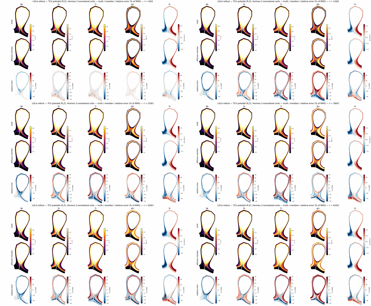
A physics check we care about is transport. The radial-flux PDF is strongly non-Gaussian and intermittent, and the LOLA members broadly reproduce that shape. Kurtosis is only a rough summary and is sampling-dependent, so we give the range rather than one figure: on the full c5 evaluation truth and member are close (both of order ~84, against a Gaussian value of 3); on the earlier c4 run the member overshot (~113 vs truth ~84, i.e. too intermittent); and on the reduced mid-plane slice plotted in Fig 7 both sit near 65–70. The stable statement is just that member and truth are both far from Gaussian and of similar order — not a precise match. The flux profile tracks truth (L1 ≈ 1.3×10⁻⁴), and member FreezeRatio is roughly flat in τ (about 0.7–1.2 from τ=32 to 63) in these runs, with little rollout decay.


8Two ceilings we can name
Two limits remain. Representation. A note on units first: n is the full-torus toroidal mode number, and because the simulation is a 1/5-torus wedge (zperiod=5) it only represents n in multiples of 5 (an in-wedge harmonic k maps to n=5k). So the 88-cell toroidal axis carries in-wedge harmonics up to 44, i.e. up to n≈220. The isotropic f8 latent compresses those 88 cells to 11 (in-wedge Nyquist ≈5, i.e. n≈25 in principle), and with codec blur the hard edge density mode near n=35 (in-wedge k=7) survived only to about n≈10. An anisotropic autoencoder (z44: 88→44, striding the periodic axis less) has ample headroom and does preserve that mode on round-trip. But the trained dynamics did not follow: the z44 rollout still reverted the edge peak to n≈5 and kept only about 31.5% of the truth's edge toroidal power. So the codec ceiling looks real and removable, while the residual failure seems to sit in the dynamics/training formulation rather than the representation — and validation likelihood did not flag it. (Separately, a gappy-POD check suggested the f8 latent behaves like a spectral low-pass: physical-space reconstruction kept high-k coherence ~0.23, while quantities routed through the latent fell toward a free-model floor ~0.05 — a likely reason pointwise-RMSE "gains" can just be the freeze rewarding blur.)
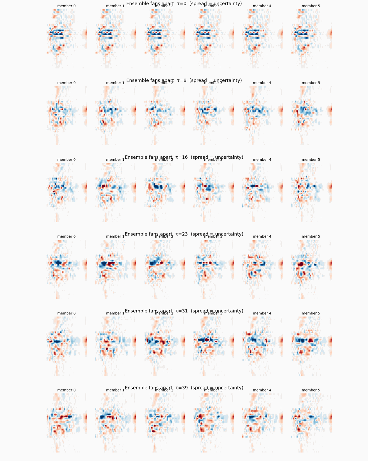
Distribution. The ensemble is under-dispersed (spread-skill roughly 0.3–0.6 across fields and lead times; want ~1), and the deficit sits at the large scales (low-k SSR ≈ 0.29 for φ on the c4 per-k run). There is a related tension worth stating plainly: individual members are slightly over-energetic on some fields (FreezeRatio(φ) ≈ 1.1–1.15, i.e. ~20–30% too much increment energy, above the AE round-trip ceiling), while the ensemble as a whole is under-dispersed. Together those point to members sharing a common error direction — the usual signature of a miscalibrated diffusion ensemble — so FreezeRatio is best read as |FR−1|, a tripwire against the freeze rather than a skill score. We traced part of this to the sampler and part to a genuine amplitude deficit, and addressed the amplitude piece with a held-out per-mode inflation. Calibration is not solved.


9Where this leaves us
A compact summary of what we saw. Every entry is single-trajectory and preliminary; the FreezeRatio(ω) column mixes runs (c4/c5) and should be read as an order-of-magnitude, not a leaderboard.
| Family | Objective | FreezeRatio (ω) | What we saw |
|---|---|---|---|
| ViT3D (deterministic) | pointwise MSE/L1 | ~0.20 | froze in our runs; capacity & time-stride did not lift it |
| GAOT / MAGNO | all-to-all, geometry graph | 0.03→0.11 | mismatch (memory, overfit); the objective looked like the useful part |
| JEPA / VICReg | predictive SSL | latent freeze | dropped high-k, seemingly by design; maybe a global-estimator, not a generator |
| Conv-AE (reference) | reconstruction | ~0.94 | the substrate: keeps the field, but has no dynamics of its own |
| LOLA (latent diffusion) | generative ensemble | ~0.7–1.2 | kept small scales & broadly the transport statistics, in these tests |

A tentative pattern: it may be less about the block diagram than about matching the objective and the representation. A pointwise loss rewards the mean; a point-cloud tokenizer can discard a known grid; a predictive latent seems to keep only the predictable. In our tests the one family that stayed off the floor was the generative one, sampling the conditional distribution rather than reporting its mean, which seemed to avoid all three. We would not call it a finished emulator: it is one trajectory, the ensemble is still under-dispersed, and the dynamics ceiling of §8 is open. What we can say is that, of the things we tried, generation in a reconstructive latent is the direction that looks worth pushing on next.
References
- R. Green, Z. S. Abdallah, T. M. Silva Filho, Expectations vs. Realities: The Cost of MSE-Optimal Forecasting Under Conditional Uncertainty, KDD 2026, arXiv:2606.04342.
- C. E. Leith, Theoretical Skill of Monte Carlo Forecasts, Mon. Wea. Rev. 102, 409–418 (1974).
- F. Rozet, R. Ohana, M. McCabe, G. Louppe, F. Lanusse, S. Ho, Lost in Latent Space: An Empirical Study of Latent Diffusion Models for Physics Emulation, arXiv:2507.02608.
- M. McCabe et al. (Polymathic AI), Walrus: A Cross-Domain Foundation Model for Continuum Dynamics, arXiv:2511.15684.
- S. Wen et al., Geometry Aware Operator Transformer as an Efficient and Accurate Neural Surrogate for PDEs on Arbitrary Domains (GAOT/MAGNO), NeurIPS 2025, arXiv:2505.18781.
- A. Bardes, J. Ponce, Y. LeCun, VICReg, ICLR 2022, arXiv:2105.04906; R. Balestriero, Y. LeCun, LeJEPA, arXiv:2511.08544; D. Klindt, Y. LeCun, R. Balestriero, When Does LeJEPA Learn a World Model?, arXiv:2605.26379.
- J. J. van de Wetering, B. Zhu, Neural operator transformers capture bifurcating drift wave turbulence in fusion plasma simulations (all2all training), arXiv:2603.05730.
- A. Theodorsen, O. E. Garcia, J. Horacek, R. Kube, R. A. Pitts, Scrape-off layer turbulence in TCV: evidence in support of stochastic modelling, Plasma Phys. Control. Fusion 58, 044006 (2016); O. E. Garcia et al., Nucl. Fusion 47, 667 (2007).