Single simulated trajectory; synthetic (not measured) diagnostics; the observability numbers are first-pass estimates with stated limitations, not device predictions. Directional guidance, not a design basis.
1Why conditioning
On a device you get a handful of diagnostics at fixed locations, not the whole field. Future reactors make it worse: neutron damage and the breeding blanket leave very little wall for instrumentation. The strategy is to learn the field on a heavily-instrumented experiment and transfer to a frozen model — which requires knowing exactly what a realistic diagnostic set can constrain.
2The synthetic diagnostics
Each diagnostic is a differentiable forward operator on the state: a GPI/BES-like emissivity proxy (we use ε ∝ n√Te over a 10×10 outboard-midplane window crossing the separatrix; real HeI GPI scales closer to n0.4–0.6Te0.6–0.8 with a neutral-cloud factor — for a monotone observability ranking the exact exponents matter little, and we say so rather than claim fidelity), divertor Langmuir (Isat ∝ n√(Te+Ti), Vfloat = φ − 2.8Te; the sheath coefficient is ~2.8–3.2 for deuterium, TCV uses 3.0), and a reflectometry chord. Placed at one toroidal plane they touch ~0.1% of the grid cells (~0.02% of the five-field state values).
These are faithful to the machine, not invented. TCV carries a midplane gas-puff-imaging system (a 10×12 avalanche-photodiode array on a single toroidal port, ~50×40 mm, 2 MHz), a second GPI camera at the X-point/divertor, and >180 wall-embedded Langmuir probes plus reciprocating midplane and divertor probe arrays. Critically for what follows, the coverage is asymmetric: density and electron temperature are richly measured by fast diagnostics, while potential and parallel flow are seen only by Langmuir probes, and ion temperature has no fast diagnostic at all (only charge-exchange spectroscopy, at profile speed). A cited breakdown of the full suite and the sheath/emissivity relations is in the companion diagnostics reference.


3The anchored rollout
A free rollout drifts from the true trajectory (chaos); an anchored rollout ingests sensor readings at intervals and pulls the ensemble back. We tried two forms of the pull: an ensemble-Kalman (ETKF) update, whose weight is set by the ensemble spread (which is why the calibrated prior of Notebook I matters, and which here needed inflation 5.0 to act at all), and a variational fit through the decoder with a fixed prior weight. The storyboard below is the variational form; the anchoring curve is the ETKF form.

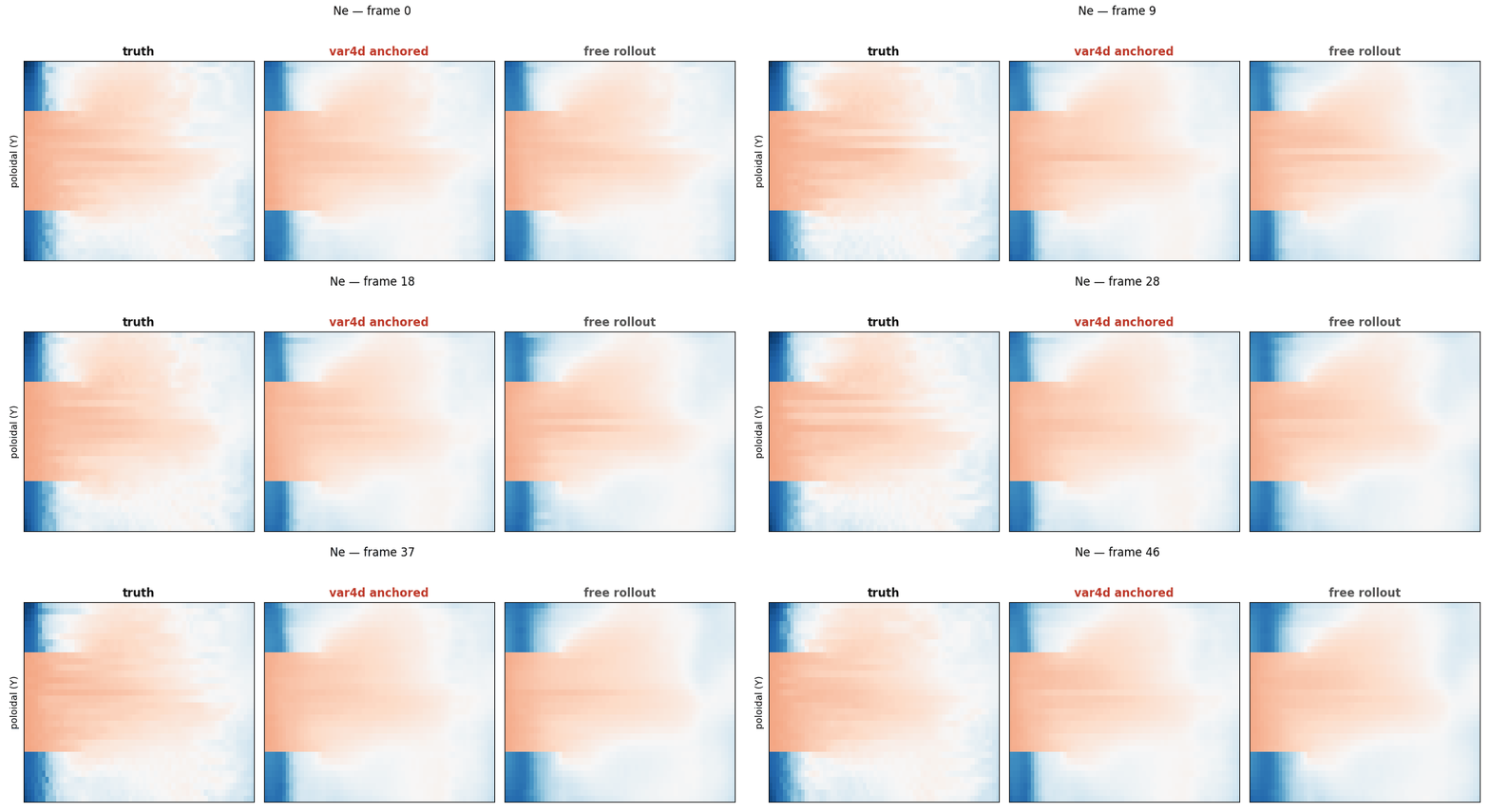

The honest result. With near-full coverage the anchor holds the trajectory's error bounded (it does not drive it to zero). With the realistic one-plane, edge-only suite, global ensemble-mean error is not reduced. The reason does not appear to be that the method is wrong — it looks like a statement about information and filter capacity, which we try to make precise next.
4Three misleading signals, and how we caught them
A false positive (a learned head). A learned analysis head reported large error reductions (1.35× early; 1.62× on a corrected-geometry retrain) — but on one trajectory such a head can minimize its loss equally well by memorizing this shot's drift. The decisive test is cross-shot: feed it observations from a different discharge (85604 obs → 85606 forecast). Its gain survived that (cross-shot penalty 1.0025 vs a 1.01 bar) and survived time-shuffled observations (1.0042), and vanished only when observations were removed — the signature of keying on innovation presence, not content. It replayed a trajectory rather than assimilating. Closed.
A false negative (a rank-starved filter). A 16-member ensemble-Kalman filter can correct only 15 directions and collapses the ensemble on the first update. Its ~1× global result is a rank signature, not absent information — but see the next trap.
A subtler trap (rank was not the whole story). Re-running the filter at 64 and 128 members did not help. The ensemble is under-dispersed at analysis time (proper spread-skill ~0.2–0.4), so the Kalman gain under-weights the observations at any rank. The binding constraint is prior calibration, not filter capacity — and, as the methods note explains, that calibration is structural: the generator’s per-step variance is fixed by its noise schedule, not learned, so no inference-time lever (inflation, sampler) and no fine-tune with the current loss can change it. A denoiser with a learned variance is the real fix.
5A first-pass observability estimate
Rather than iterate on filters, we estimate the observability directly: against a climatological ensemble of states drawn from the trajectory, form the noise-normalized observation anomalies for each sensor suite and take the singular spectrum (degrees of freedom for signal, Rodgers-style). Three methodological caveats, stated up front, that a careful reader should hold against the table below. (a) The ensemble is ~310 frames at stride 2, which is not fully decorrelated against the slowest field (τcorr(φ) ≈ 11 frames); DFS is bounded by ensemble rank (at low observation noise it saturates there, ~308), so the table below quotes the obs-noise = 1.0× channel-std row, where DFS sits well below the rank bound. Even so the counts are upper-bound-flavored and partly reflect sample size; a decorrelated re-run is the needed follow-up. (b) The synthetic GPI here observes its 10×10 window on all toroidal planes — far more toroidal coverage than a real single-port GPI — so the estimate is generous to the sensors; notably, the pessimistic conclusion below survives even this generosity. (c) The toroidal-band energy split is computed over the top-10 constrained directions, not all of them.
| GPI toroidal coverage | constrained directions (DFS, noise 1.0×) | note |
|---|---|---|
| single port (real GPI: one 2D poloidal image) | ~11–14 | stride-robust; ~40–45 at noise 0.1×. The physical number. |
| all 88 toroidal planes (idealized) | ~185 | sample-limited (DFS/N → 0.95 as the ensemble shrinks) — retired as a measurement |
A correction we owe the reader: the "~185 directions" from an earlier draft is an artifact — a real GPI is a single toroidal port (a 2D poloidal image; TCV's midplane GPI is a 10×12 array on one port [see the diagnostics note]), and the all-88-plane version was unphysical, its DFS chasing the ensemble rank. The honest single-port number is ~11–14 constrained directions at realistic noise. What survives, and matters: those directions are large-scale (a single port is toroidally non-selective, so it constrains local mixed-n structure, not the turbulent band). The reading is unchanged in spirit — the turbulent phase is not constrained by a linear snapshot; recovery must come from the prior and the dynamics through time, which is what an anchored rollout bets on.
6The deployable suite: reflectometry + divertor Langmuir
An earlier draft of this section reported larger gains and called the winning suite "GPI + Langmuir." An independent audit found three bugs in our evaluator and one mislabel: a structured-inflation term that leaked the held-out truth, an improper spread-skill statistic, an unpaired free-vs-anchored comparison, and the wrong sensor name. We fixed the evaluator (leak-free inflation off, common-random-number pairing, proper per-field spread) and re-ran on the base model across three held-out windows. The numbers below are the honest, corrected ones; the direction held, the magnitudes and the sensor identity did not.
The observability analysis says a single port sees the large scales, not the phase, and that the sparsely-covered fields (potential, ion temperature, parallel flow; see the diagnostics note) are the ones at risk. So we ran the anchored rollout on progressively richer sensor suites, on the held-out shot at three untouched starts, scored on the transport-relevant large scale (n=0): does adding the diagnostics TCV has actually recover the unobserved fields?

The corrected result still holds, and it is robust across three held-out windows. A single density diagnostic, alone, does not anchor the transport state (every field below 1 — one 2D window cannot constrain the whole cross-section). Adding a potential (divertor-Langmuir) channel recovers most of it: density ≈1.5×, parallel flow ≈1.5×, potential ≈1.3×, ion temperature ≈1.05× (carried by the emulator’s learned cross-field structure, since no sensor observes it) — while electron temperature worsens (≈0.9×), the one field this suite does not help. The effective minimal suite is midplane reflectometry (density) + divertor Langmuir (potential), both of which TCV fields; global error drops ~13% (mean) / ~24% (final).
Two honest caveats. (1) These are transport-scale (n=0 edge) gains, not global — deliberately, since the observability analysis says that is the constrainable subspace and global RMSE just re-measures the unanchorable turbulent phase. (2) Even with the corrected evaluator, the ensemble is under-dispersed: proper spread-skill is ~0.2–0.4 across suites (the reflectometry+Langmuir suite is best, ~0.37). That under-dispersion is not fixable at inference or by our current fine-tune, for a structural reason given in the methods note — the generator’s per-step variance is fixed by its noise schedule, not learned, so there is no calibrated dispersion for a filter or a sampler to use. A denoiser that outputs a learned variance is the real next step.


Two caveats keep it honest. Sparsity matters: the dense edge array over-observes and the under-dispersed gain overshoots the observed density (~0.72–0.77×, i.e. worse than free) — the sweet spot is the sparse pair, not more channels. And calibration still binds: this is why the dense suite hurts, and why the durable next step is the trained dispersion fix (Notebook I’s per-mode inflation, then an all-to-all / fair-CRPS fine-tune) — only then does adding coverage pay off cleanly. Ion temperature has no fast diagnostic on TCV at all (only charge-exchange spectroscopy, slow), so its ~1.0 here is the ceiling of what cross-field inference alone can do.
7Layered observability, and the working target
| Layer | Observable? | Why |
|---|---|---|
| Large-scale / transport (profiles, mean flows, separatrix, divertor loading) | yes (order 10² DOF, this estimate) | SOL two-point coupling + cross-field constraints; low-dimensional |
| Turbulent phase on sensor-connected flux tubes | only with capacity | plausibly observable; beyond a 16-member filter |
| Turbulent phase in unconnected regions | not from a snapshot | chaotic, decorrelates quickly; any recovery must come from prior + dynamics over time |
Our working target is a calibrated posterior of the large-scale transport state — reconstructed first from the coupled multi-sensor suite (a nonlinear, calibrated generative reconstruction that may generalize better than a linear basis, though regime shift remains the hard limit), then anchored. Pointwise turbulent-microstate reconstruction looks like the wrong objective here. The directional statement — "a realistic diagnostic set appears to constrain order-10² modes of transport state, and very little of the turbulent phase, in a single snapshot" — is the useful output, and it frames what added coverage or a higher-capacity filter would buy. It should be re-derived with a decorrelated ensemble and a single-port GPI before being used for anything quantitative. Paper I's per-mode inflation is the kind of prior such a filter needs.
Methods note
Observability from the SVD of the noise-normalized ensemble observation-anomaly matrix (degrees of freedom for signal + Shannon information); climatological ensemble of ~250–310 frames at stride 2 (not fully decorrelated against τcorr(φ) ≈ 11 — a decorrelated re-run is the planned follow-up); toroidal-band energy split computed over the top-10 constrained directions; GPI operator idealized to all toroidal planes; nested suites, per-channel noise 0.1–1.0× signal. Filter gains, when used, are scored per-region and per-band with held-out-sensor cross-validation rather than global RMSE (the freeze metric).
References
- H. Chung, J. Kim, M. T. McCann, M. L. Klasky, J. C. Ye, Diffusion Posterior Sampling for General Noisy Inverse Problems, ICLR 2023, arXiv:2209.14687.
- F. Rozet, G. Louppe, Score-based Data Assimilation, NeurIPS 2023, arXiv:2306.10574.
- P. C. Stangeby, The Plasma Boundary of Magnetic Fusion Devices (IoP, 2000), Ch. 5 (two-point upstream–target coupling) and §2.6 (sheath / floating potential).
- G. Evensen, The Ensemble Kalman Filter: theoretical formulation and practical implementation, Ocean Dynamics 53, 343–367 (2003); C. D. Rodgers, Inverse Methods for Atmospheric Sounding (World Scientific, 2000), degrees of freedom for signal.
- S. J. Zweben, J. L. Terry, D. P. Stotler, R. J. Maqueda, Gas puff imaging diagnostics of edge plasma turbulence in magnetic fusion devices, Rev. Sci. Instrum. 88, 041101 (2017).
- W. Biel et al., Diagnostics for plasma control – From ITER to DEMO, Fusion Eng. Des. 146, 465 (2019).
- F. Rozet et al., Lost in Latent Space (the LOLA prior), arXiv:2507.02608.