Longer-data reconstruction, fluctuation fidelity, diffusion, shot transfer and OMP-to-divertor inference. Results since October 9, with earlier controls retained where needed.
The five findings
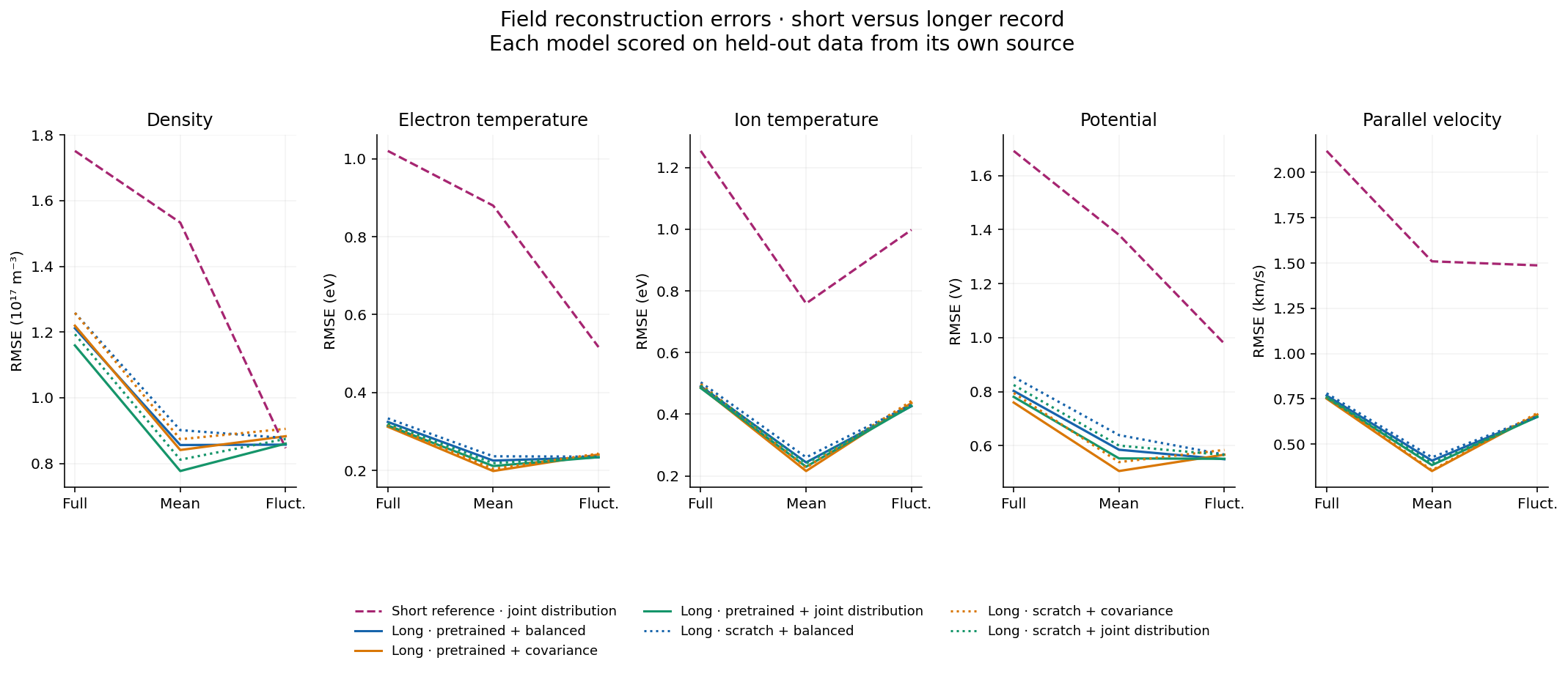
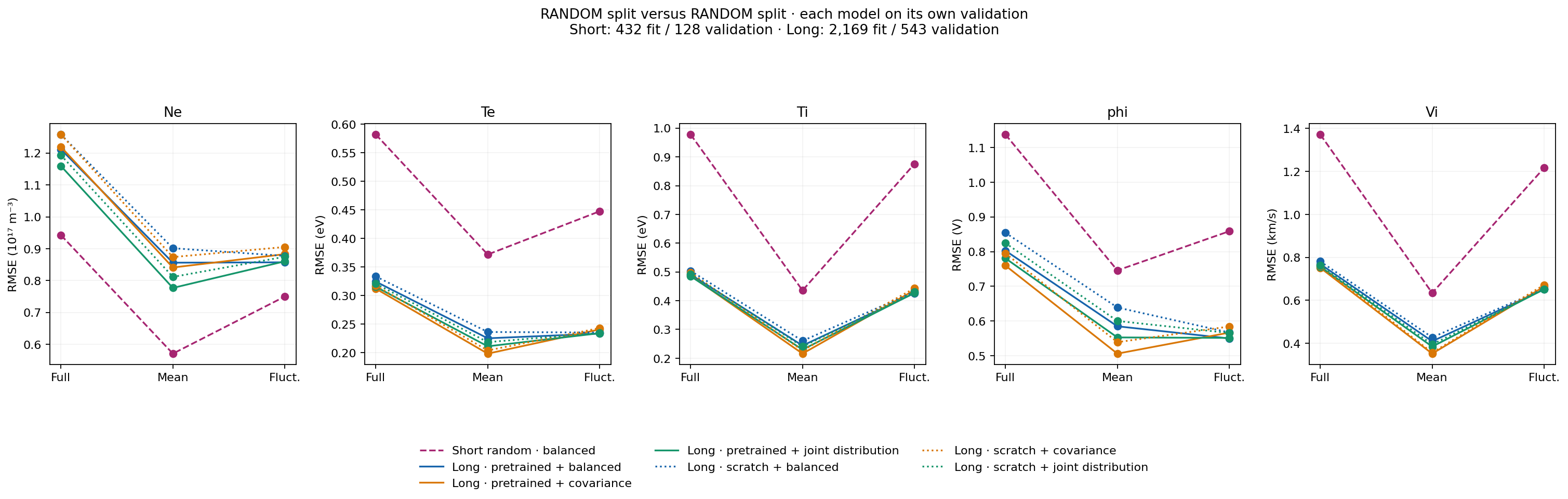
Long-data reconstruction: pretrained balanced leads the five fluctuation errors within the six matched long-data runs. The old/long overlay is a comparison across source records, not a controlled estimate of data scaling.
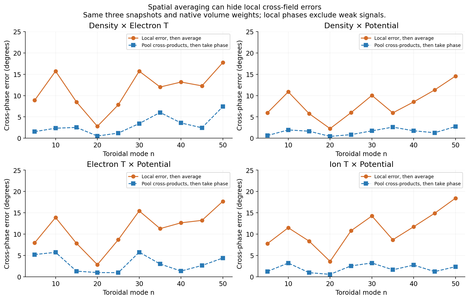
Fluctuations: matching power or pooled cross-phase can hide local amplitude and phase errors. We now show those separately.
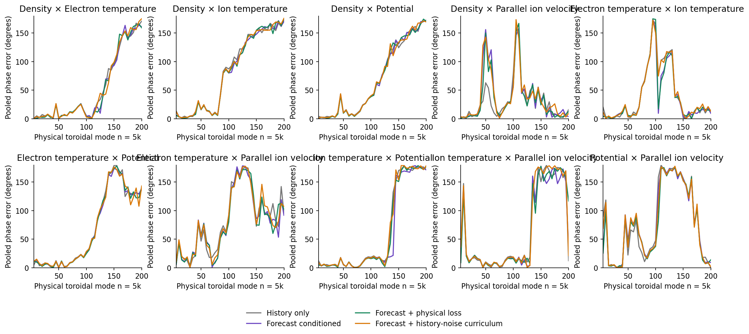
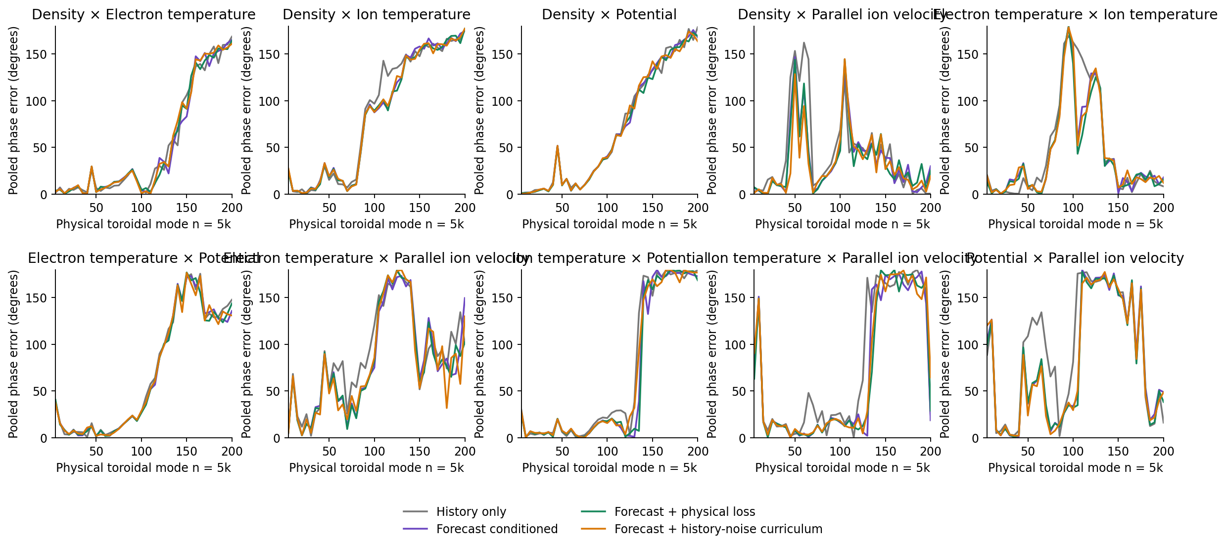
Diffusion: forecast conditioning helps; history noise trades better particle transport against worse target heat. Local realization fidelity remains unresolved.
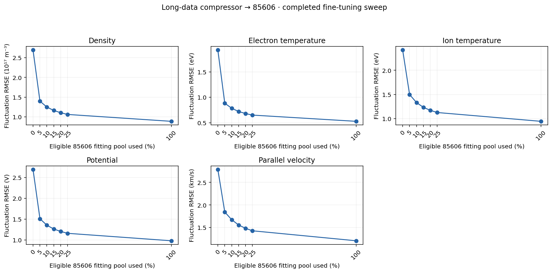
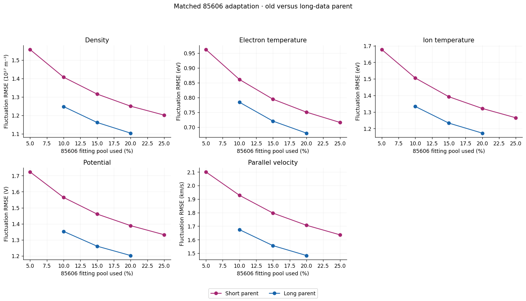
85606: all fine-tuning fractions completed; more target data continues improving all five fluctuation errors.
XY → divertor: XZ-task pretraining finished, but the physical patch still does not match full-XZ input accuracy. Target-only errors are less severe than downstream-volume errors.
Arrows are weight inheritance except the chronological model → temporal preparation dependency. Scratch long-data models have independent initialization. Click a branch to see its comparison. Complete historical tree and configuration archive.
1. Longer data versus shorter data
Question: do more data and different reconstruction objectives preserve more of the plasma state?
Five-field full volume→Trainable convolutional encoder→22,528 latent scalars→Trainable decoder→Same-time five-field volume
Family
Initialization and objective
Data and updates
Evaluation
Short reference
Earlier compressor → joint-patch distribution continuation
Legacy 85604; +6,400 updates
Legacy frames 500–623
Long six-way comparison
Scratch or earlier compressor × balanced / covariance / joint-patch loss
New 2,712-frame record; 51,200 updates each
Same 543 random-held-out frames
Chronological long control
Earlier compressor → balanced
2,169 fit; 64 guard; 479 validation
Still training; no final curve
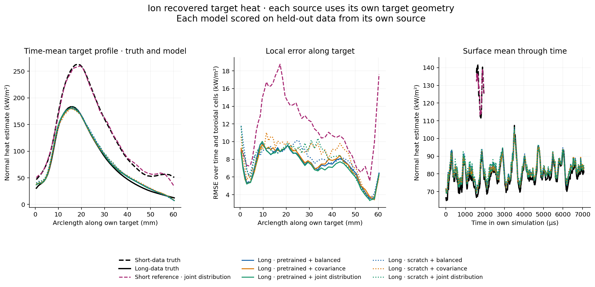
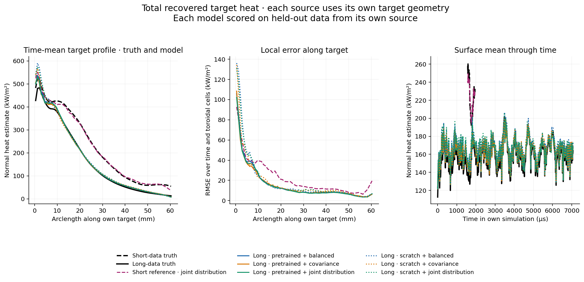
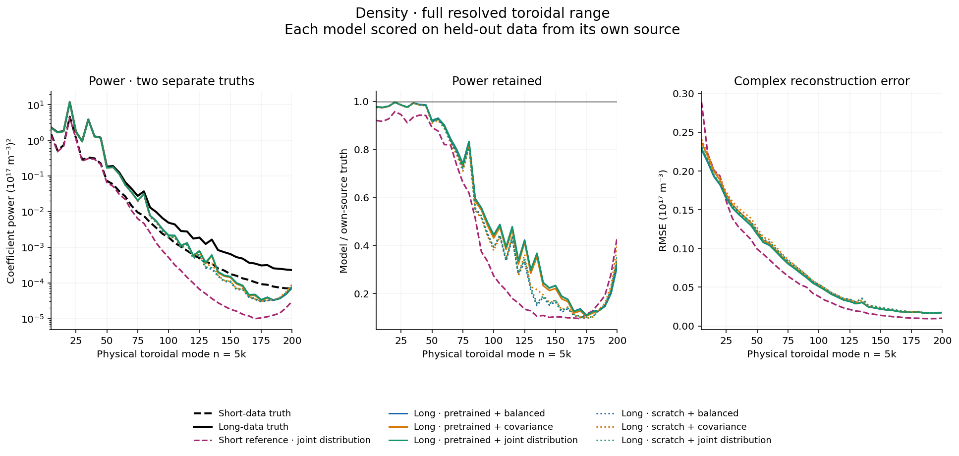
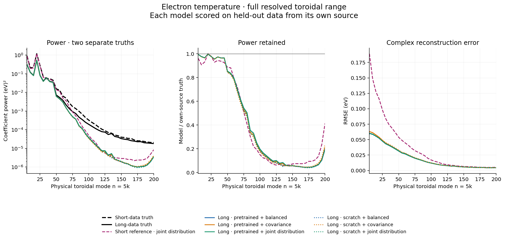
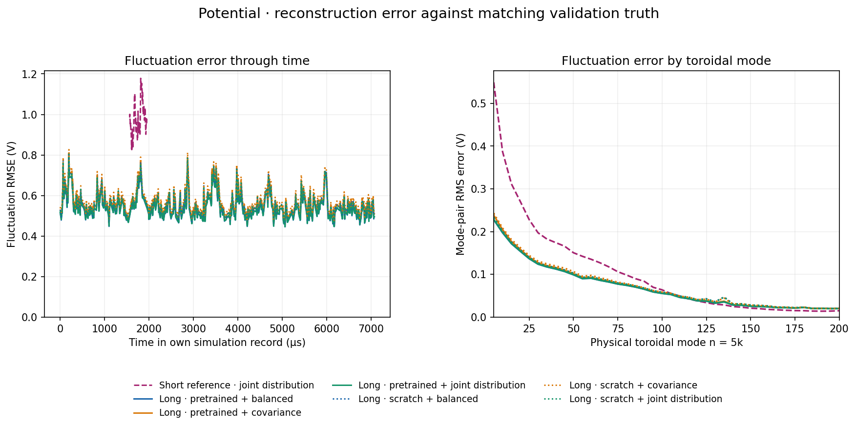
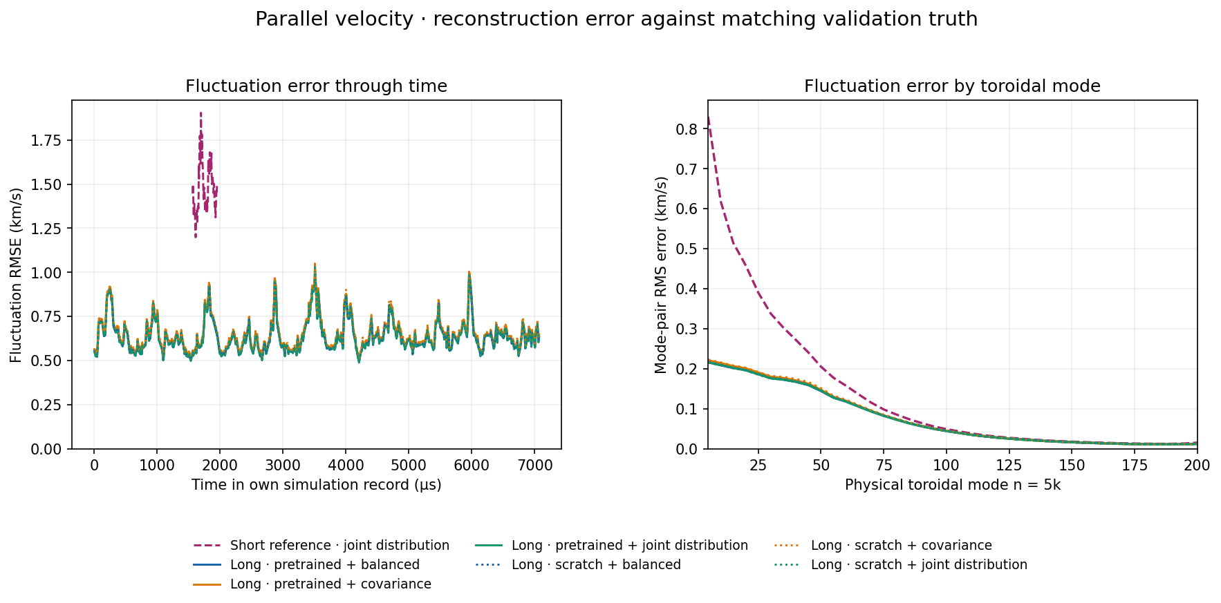
Read overlays correctly: dashed short-data curves use short-data truth; long-data curves use long-data truth. Spectra show both truths. Different source records/splits are not matched test cases. Within the six long-data models, the validation data are identical. “Pretrained” means our short-data balanced codec, not historical LoLA.
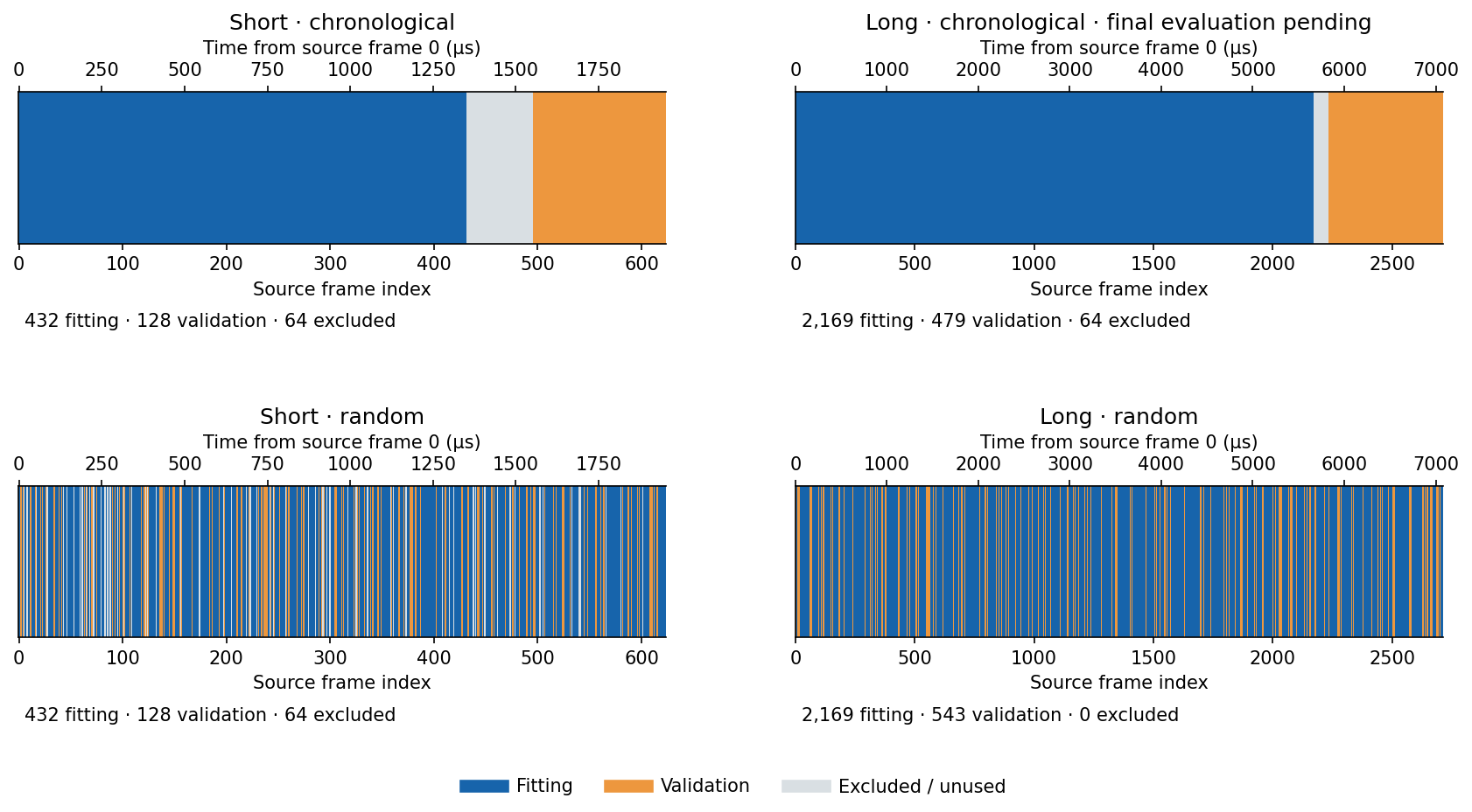
Short / long × chronological / random
Split
Short legacy record · 624 frames
Long final record · 2,712 frames
Chronological
Fit 0–431; exclude 432–495; validate 496–623. Continuation plots use 500–623.
Fit 0–2168; exclude 2169–2232; validate 2233–2711. Final evaluation pending.
Random
432 fit / 128 validation / 64 unused, scattered across 624; seed 20261008.
2,169 fit / 543 validation, scattered across 2,712; seed 20261014.
The four time splits. Blue: fitting. Orange: validation. Gray: excluded. Random unused frames are not a temporal guard. Different records have different cadences; time starts at each source frame 0. Download
Random split asks about unseen snapshots interspersed with training data; chronological split withholds a later interval. Both are reconstruction tasks with the complete target-time volume as input. Short and long models always use their own validation truth. See Section 2 for their error curves.
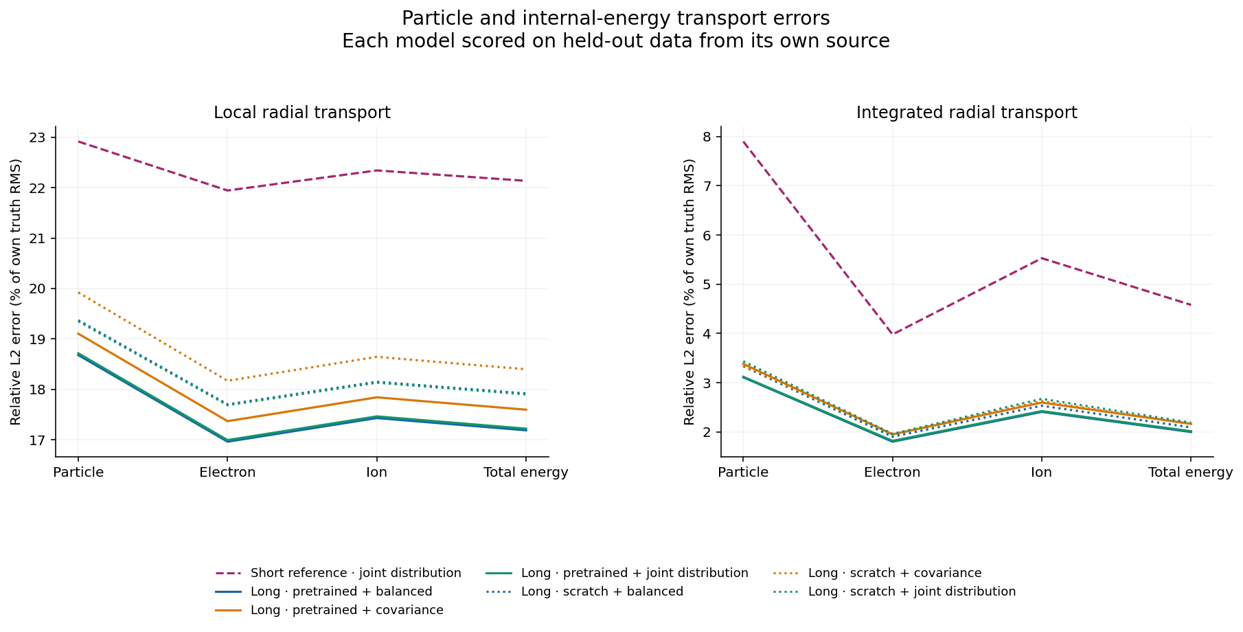
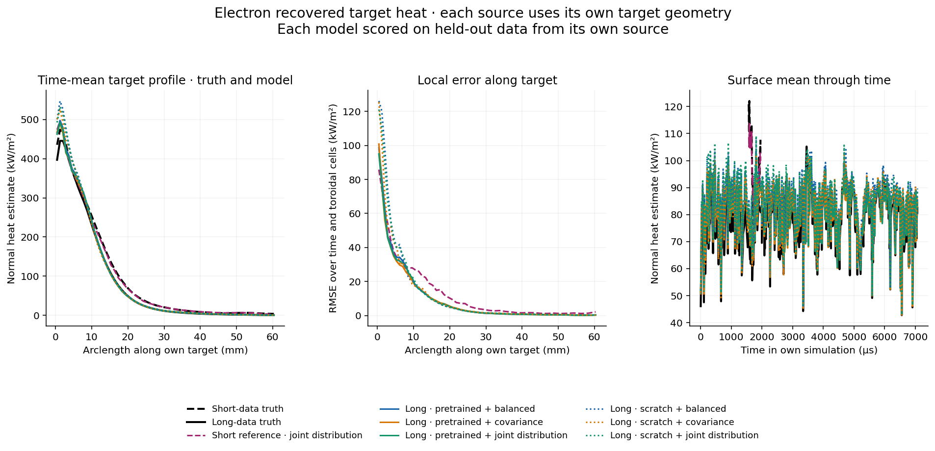
Physical errors and target heat · short reference overlaid with long models
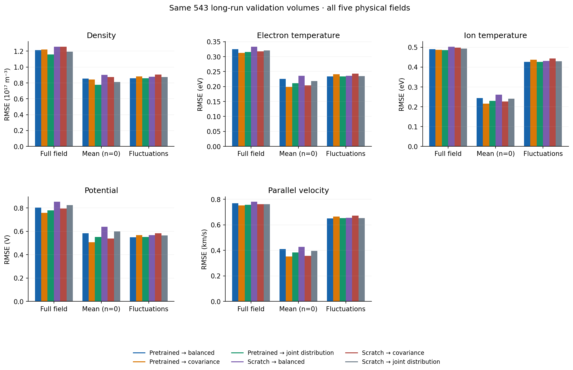
All five fields: full, mean and fluctuation errors. Own-source validation for short and long models; physical units, lower is better. Download
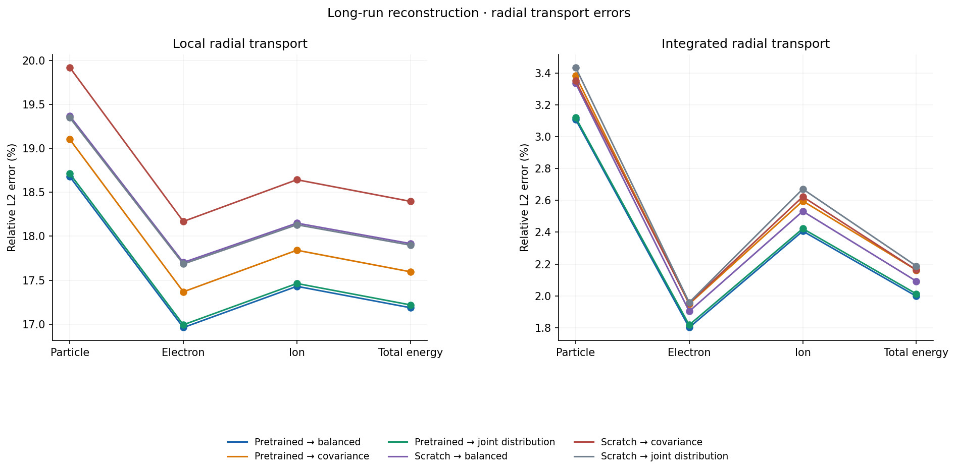
Local and integrated radial transport. Own-source truth normalization. Electron/ion internal-energy transport is not target heat. Download
Electron recovered target heat. Own-source target geometry. Recovered sheath estimate; exact new solver energy bookkeeping is not source-verified. No experimental tile-loading claim. Download
Ion recovered target heat. Own-source target geometry. Recovered sheath estimate; exact new solver energy bookkeeping is not source-verified. No experimental tile-loading claim. Download
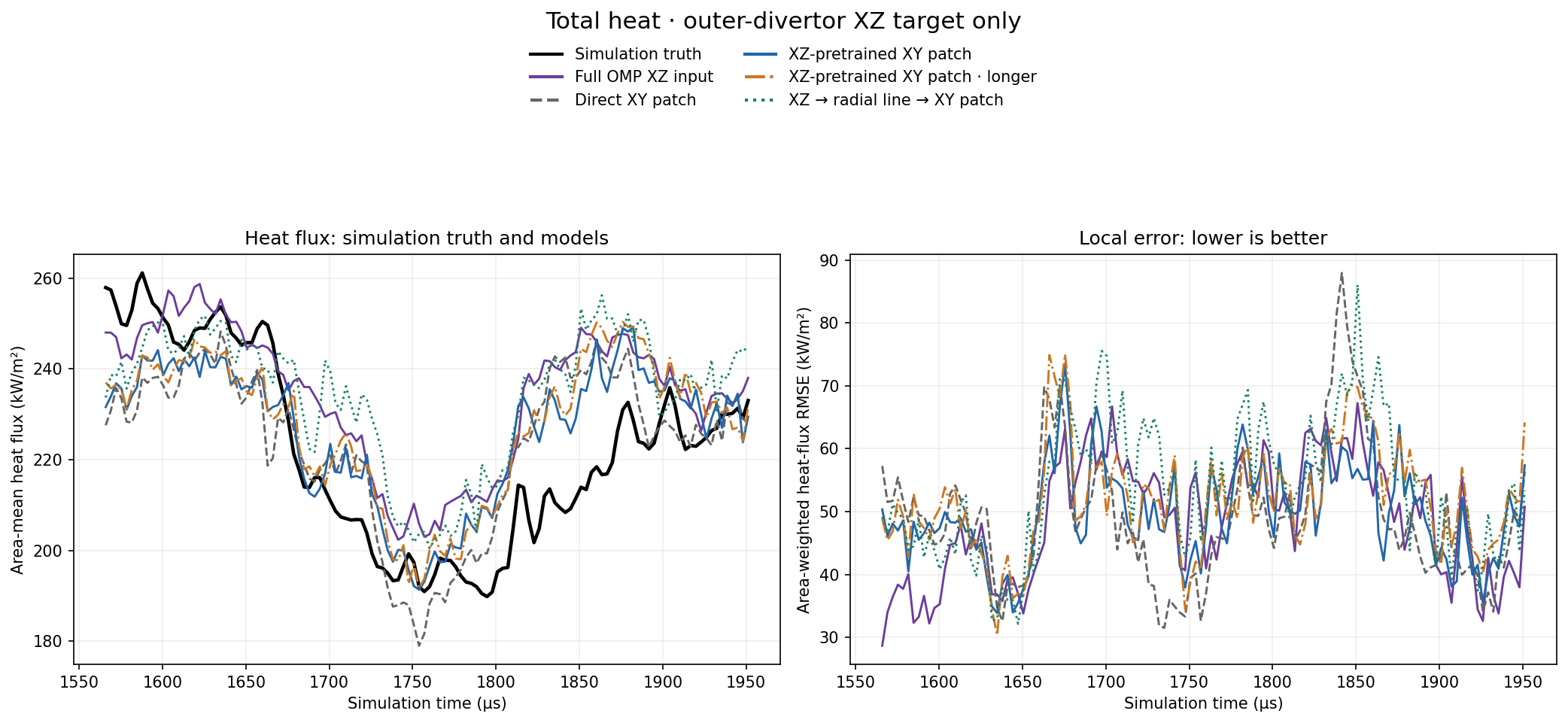
Total recovered target heat. Own-source target geometry. Recovered sheath estimate; exact new solver energy bookkeeping is not source-verified. No experimental tile-loading claim. Download
Spectra and complex errors · all five fields
Density modes. Full resolved n=5…200. Power tests amplitude; complex coefficient error also detects spatial phase mismatch. Each model uses its own source truth. Download
Electron temperature modes. Full resolved n=5…200. Power tests amplitude; complex coefficient error also detects spatial phase mismatch. Each model uses its own source truth. Download
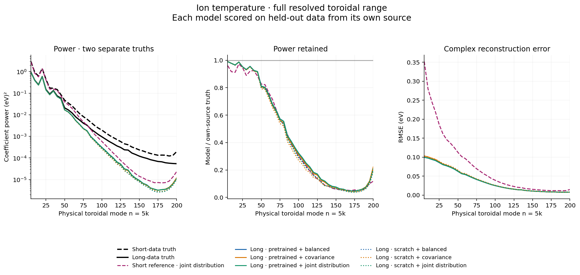
Ion temperature modes. Full resolved n=5…200. Power tests amplitude; complex coefficient error also detects spatial phase mismatch. Each model uses its own source truth. Download
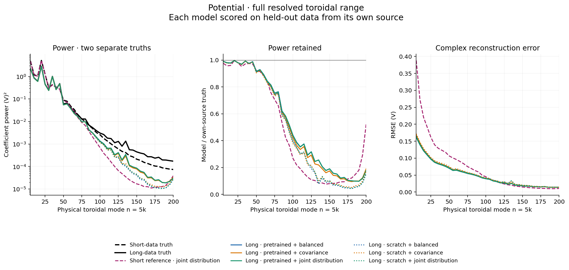
Potential modes. Full resolved n=5…200. Power tests amplitude; complex coefficient error also detects spatial phase mismatch. Each model uses its own source truth. Download
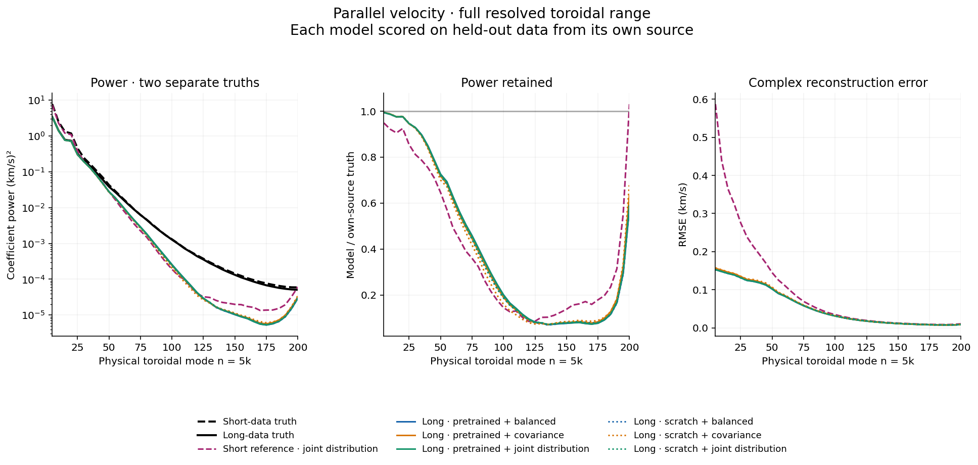
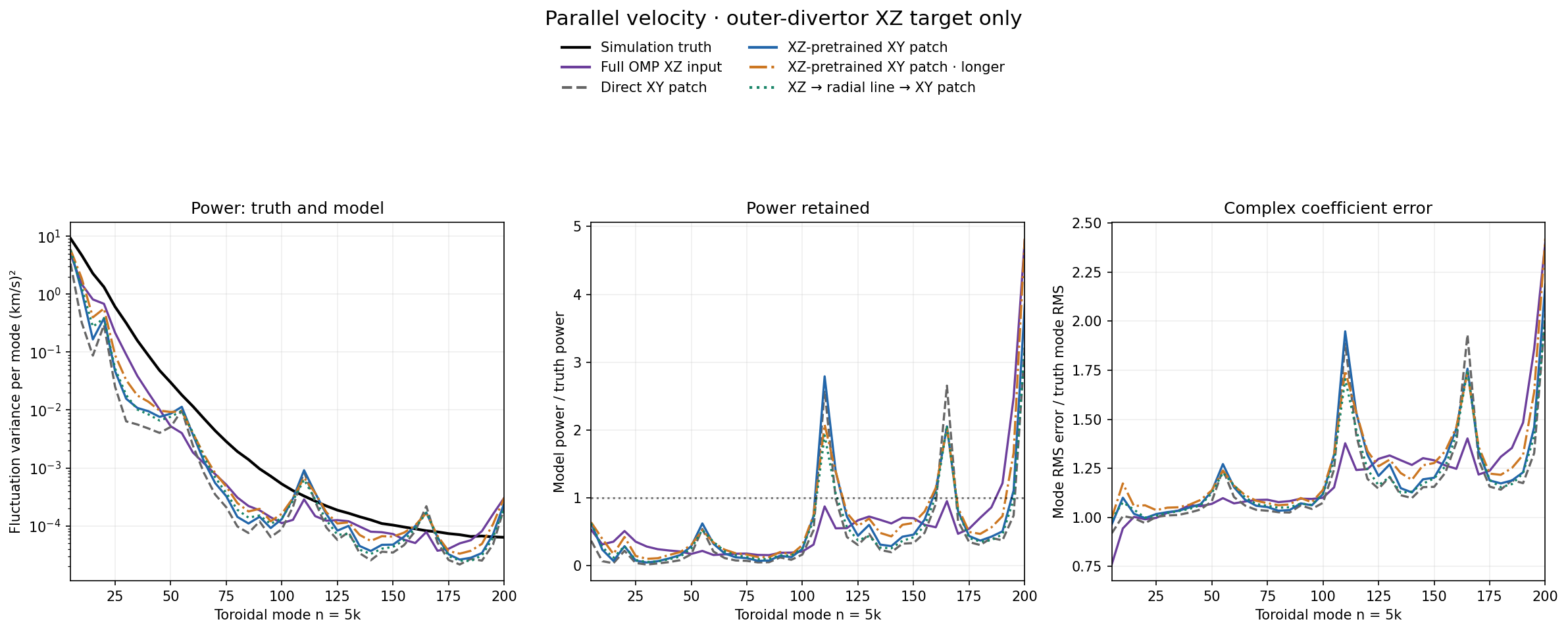
Parallel velocity modes. Full resolved n=5…200. Power tests amplitude; complex coefficient error also detects spatial phase mismatch. Each model uses its own source truth. Download
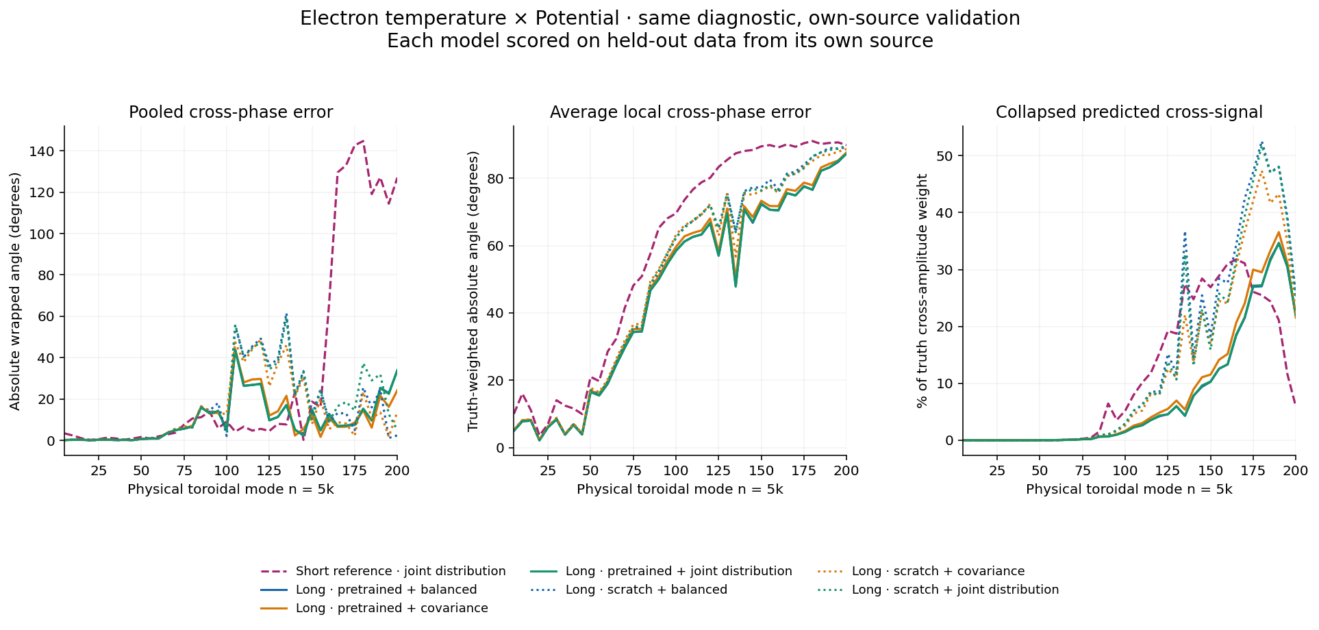
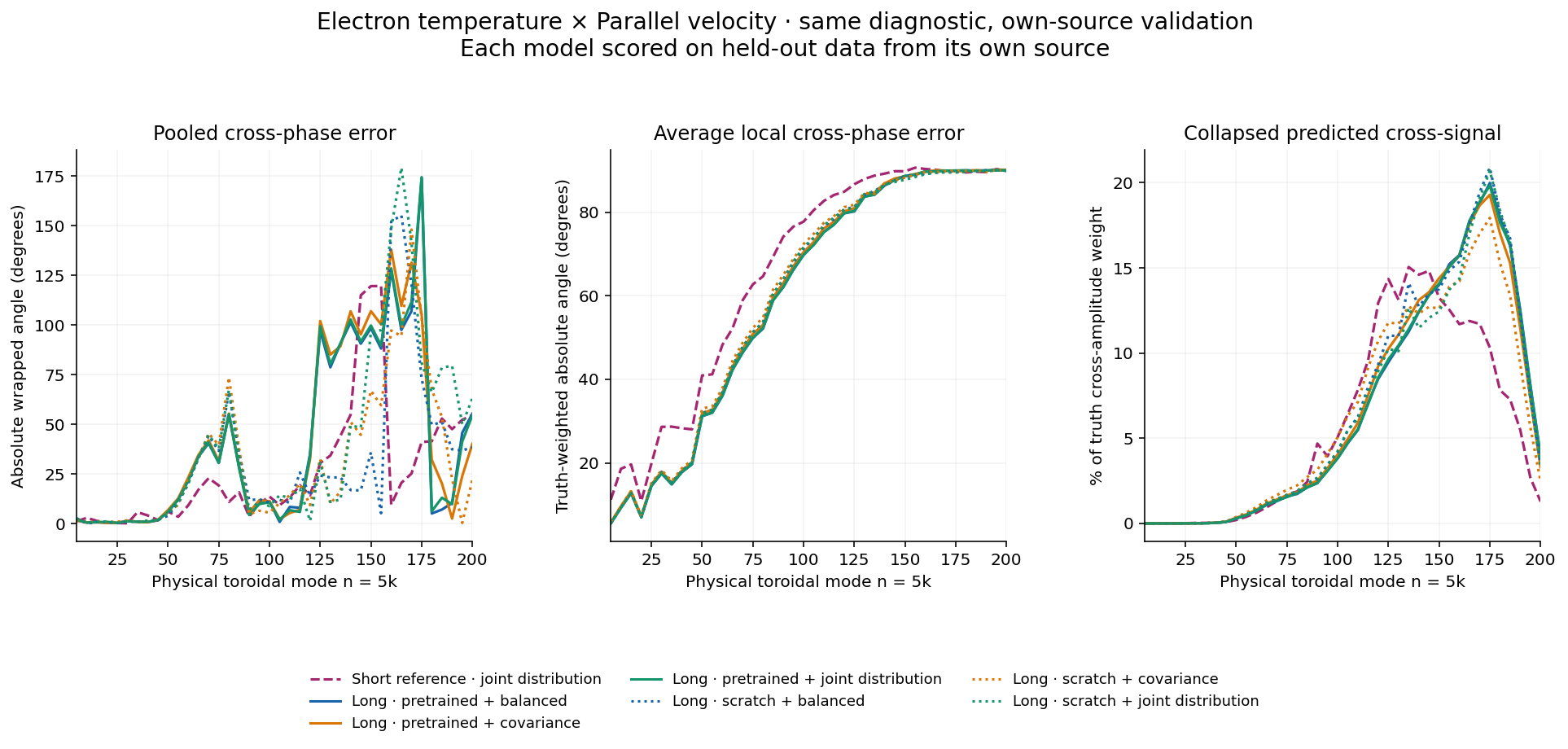
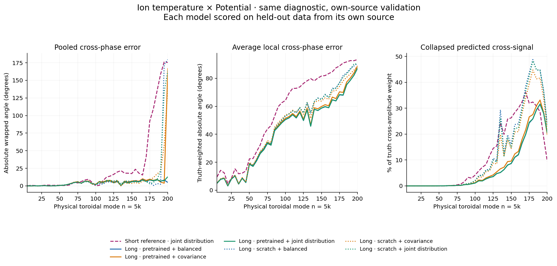
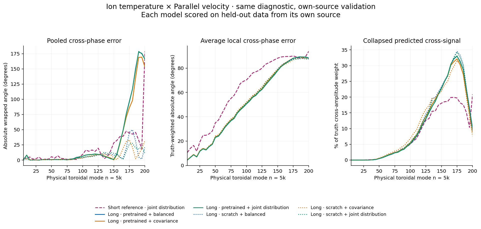
Local versus pooled cross-phase · all ten field pairs
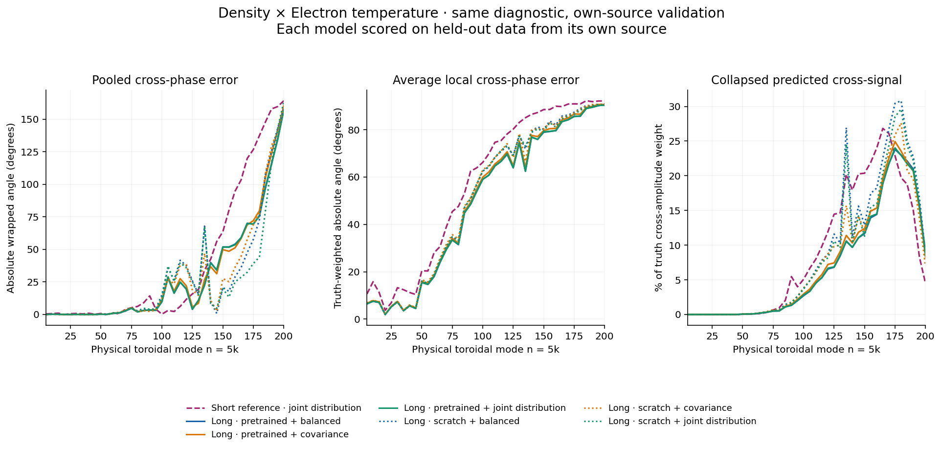
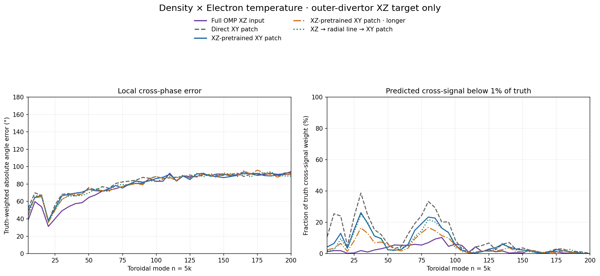
Density × Electron temperature. Local wrapped errors are calculated before averaging; pooled errors use averaged complex cross-spectra. Compare collapse coverage too; phase near zero amplitude is not reliable. Download
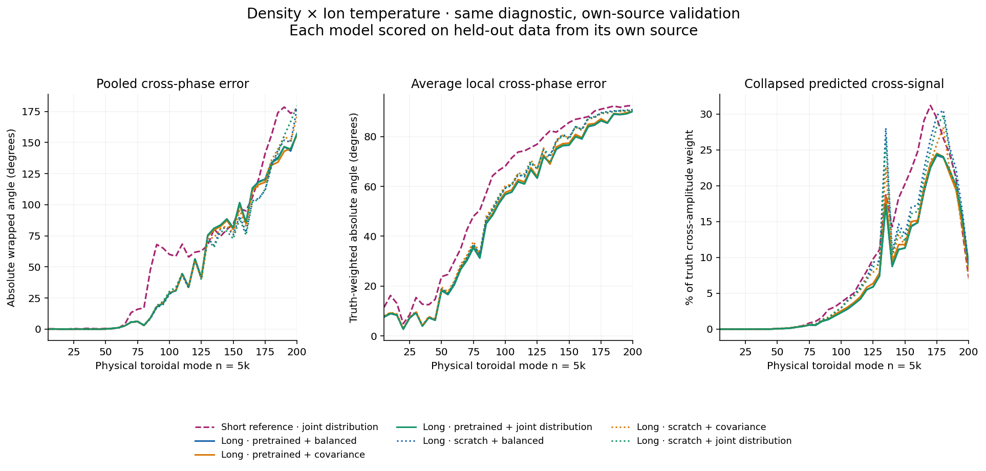
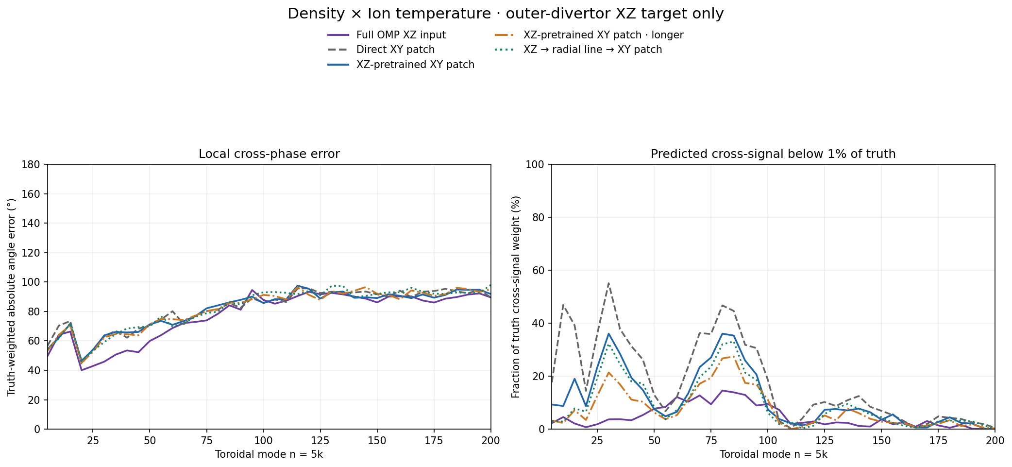
Density × Ion temperature. Local wrapped errors are calculated before averaging; pooled errors use averaged complex cross-spectra. Compare collapse coverage too; phase near zero amplitude is not reliable. Download
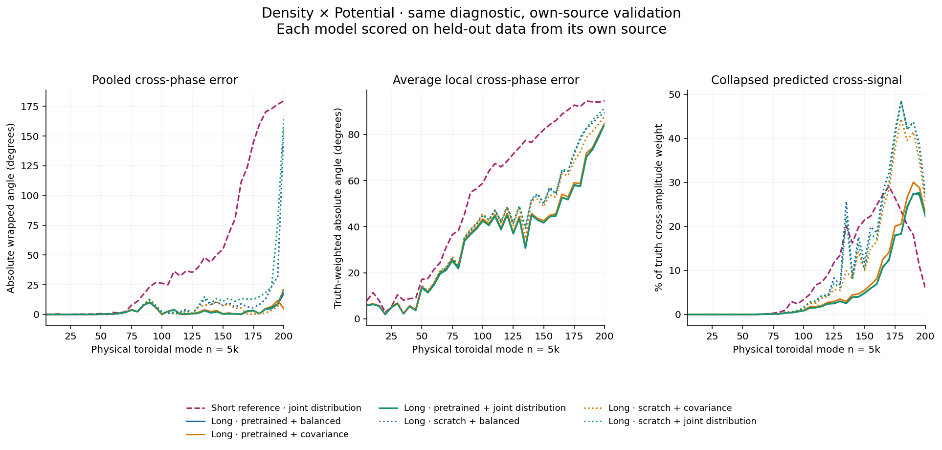
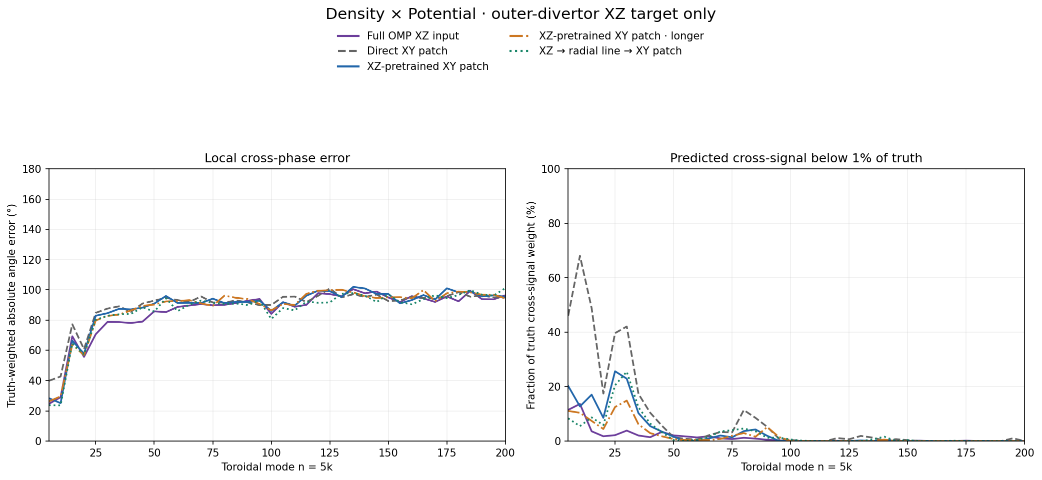
Density × Potential. Local wrapped errors are calculated before averaging; pooled errors use averaged complex cross-spectra. Compare collapse coverage too; phase near zero amplitude is not reliable. Download
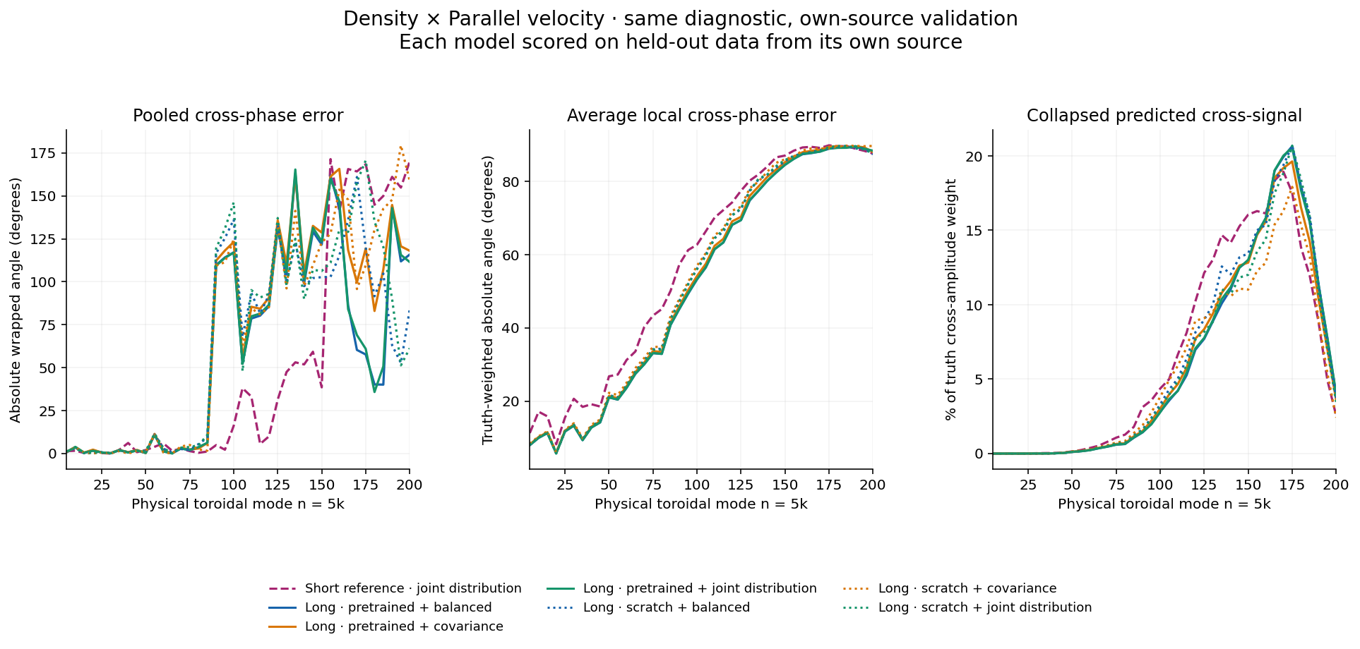
Density × Parallel velocity. Local wrapped errors are calculated before averaging; pooled errors use averaged complex cross-spectra. Compare collapse coverage too; phase near zero amplitude is not reliable. Download
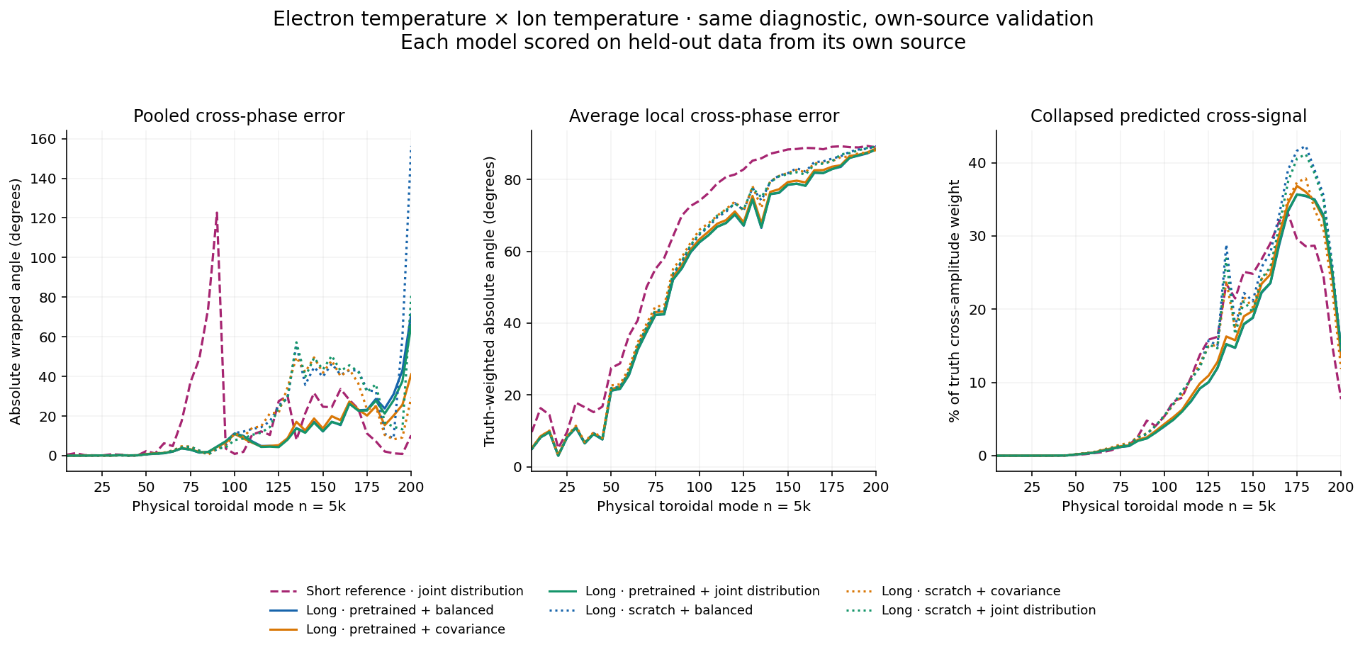
Electron temperature × Ion temperature. Local wrapped errors are calculated before averaging; pooled errors use averaged complex cross-spectra. Compare collapse coverage too; phase near zero amplitude is not reliable. Download
Electron temperature × Potential. Local wrapped errors are calculated before averaging; pooled errors use averaged complex cross-spectra. Compare collapse coverage too; phase near zero amplitude is not reliable. Download
Electron temperature × Parallel velocity. Local wrapped errors are calculated before averaging; pooled errors use averaged complex cross-spectra. Compare collapse coverage too; phase near zero amplitude is not reliable. Download
Ion temperature × Potential. Local wrapped errors are calculated before averaging; pooled errors use averaged complex cross-spectra. Compare collapse coverage too; phase near zero amplitude is not reliable. Download
Ion temperature × Parallel velocity. Local wrapped errors are calculated before averaging; pooled errors use averaged complex cross-spectra. Compare collapse coverage too; phase near zero amplitude is not reliable. Download
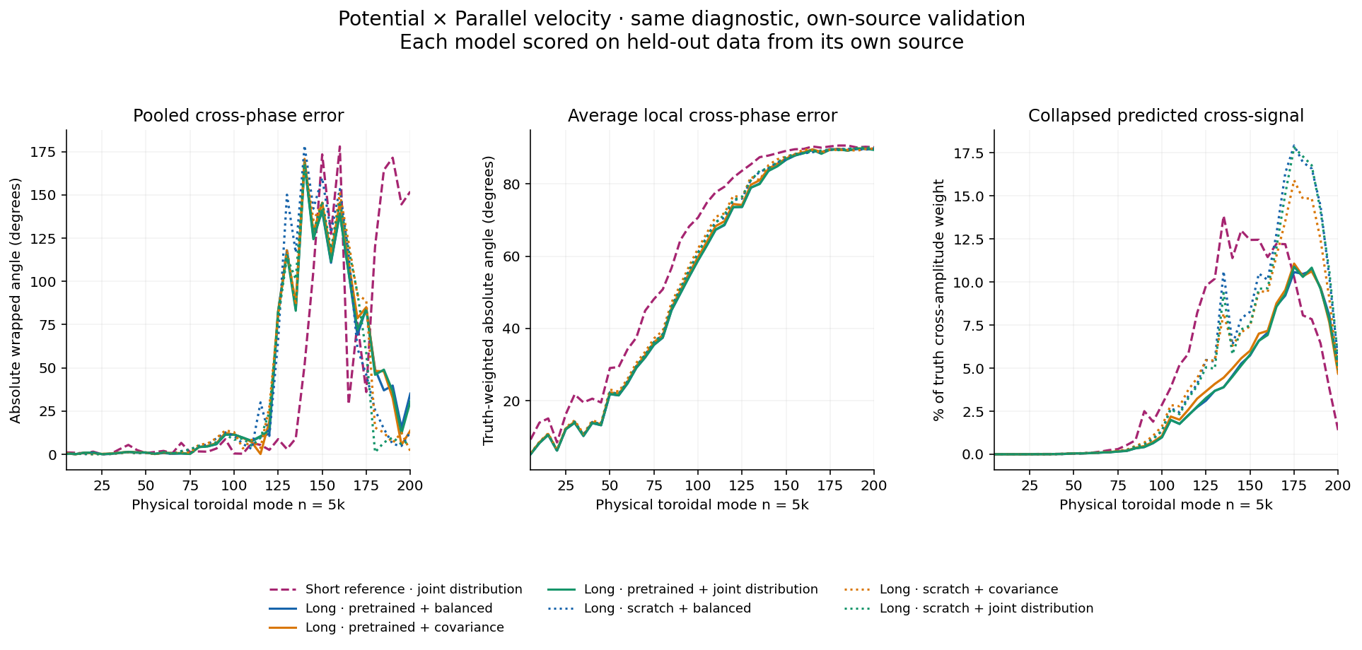
Potential × Parallel velocity. Local wrapped errors are calculated before averaging; pooled errors use averaged complex cross-spectra. Compare collapse coverage too; phase near zero amplitude is not reliable. Download
Controlled six-way long-data comparison and earlier short-data controls
Matched objectives
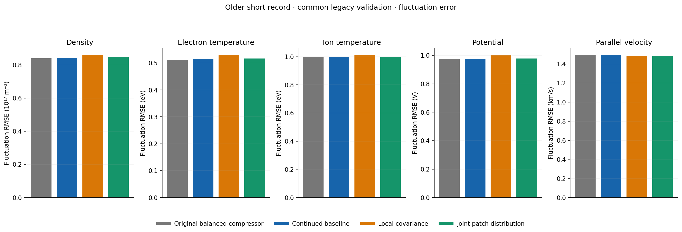
Long-data six-way field errors. All six evaluated on identical 543 volumes. Download
Long-data six-way radial transport. Common geometry, support and truth. Download
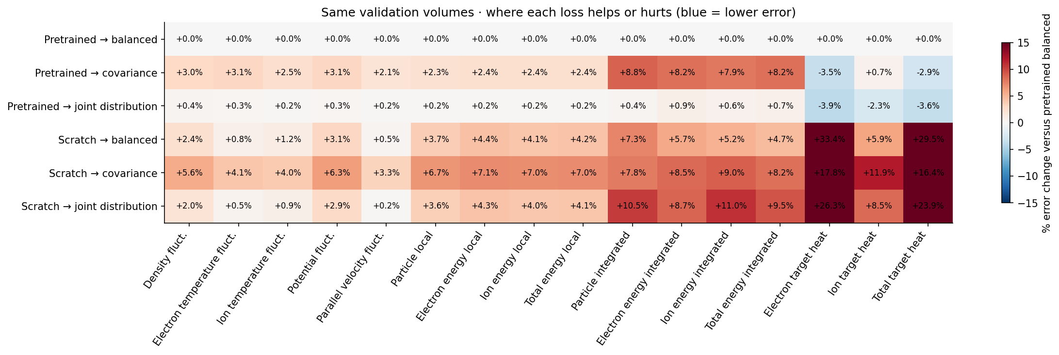
Loss tradeoffs relative to pretrained balanced. One-seed development evidence; no universal winner inferred from a single metric. Download
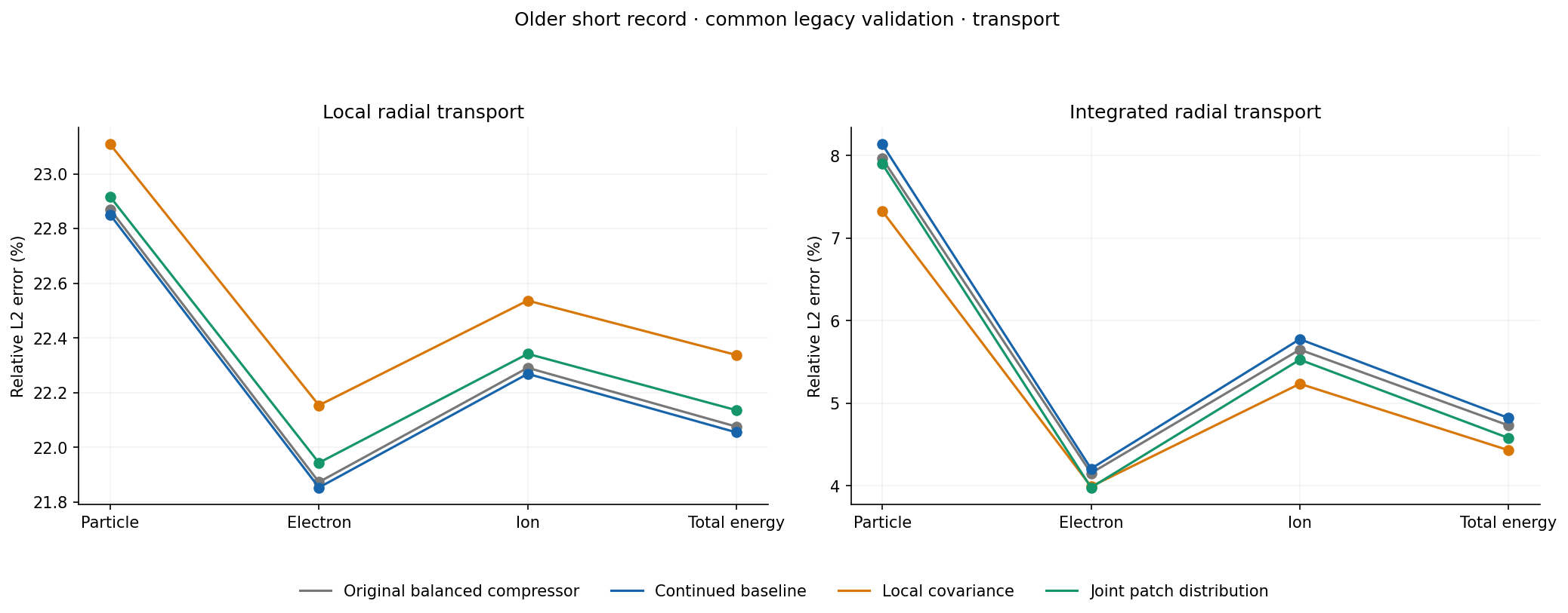
Earlier short-data transport. Original compressor versus equal-length continuations. Download
Balanced loss: equal normalized contributions from toroidal mean and fluctuations. Local covariance loss: auxiliary matching of local cross-field second moments. Joint-patch distribution loss: auxiliary distribution matching for multifield patch vectors; it does not guarantee that every reconstructed structure is in the correct place.
Shuffled versus chronological: separate experiments
Ablation
What changed
Finding
Training order
Individual frames versus four-frame bins within the same fitting interval
Chronological versus randomly assigned legacy frames
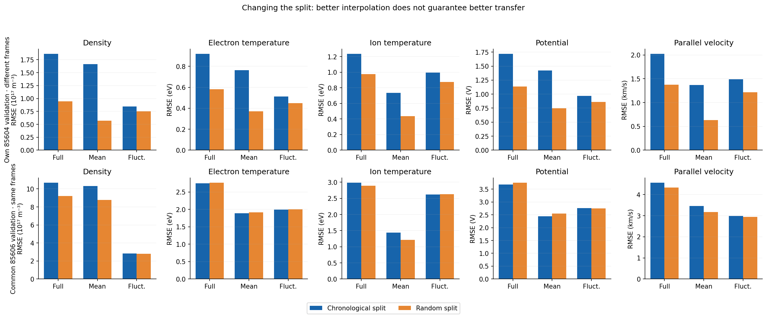
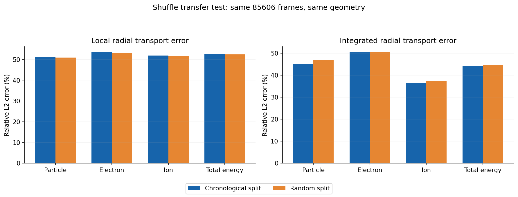
Random-split own-shot fluctuation errors were about 11–18% lower, but on different validation frames. On identical 85606 frames, differences were below 1.5%.
Short versus long, both random split
Different source records; random held-out frames in each
Descriptive comparison, not a pure data-size ablation.
Earlier split ablations
Chronological versus random split · all five fields. Top: own 85604 validation, different held-out frames. Bottom: same 85606 frames for both unadapted models; a separate cross-shot transfer test. Download
Chronological versus random · transfer transport. Same 85606 evaluation frames; distinct from own-source reconstruction. Download
Short random versus long random · reconstruction. Each evaluated against its own source truth. This short random balanced checkpoint differs from the short chronological joint-distribution reference in the other overlays. Download
Legacy fit [0,432), guard [432,496), reconstruction evaluation [500,624) here. New random split: 2,169 fit / 543 validation out of 2,712 frames; 519 validation frames are adjacent to fitting frames. New chronological control: fit [0,2169), guard [2169,2233), validation [2233,2712). Random-held-out frames are an interpolation test, not future-time forecasting evidence.
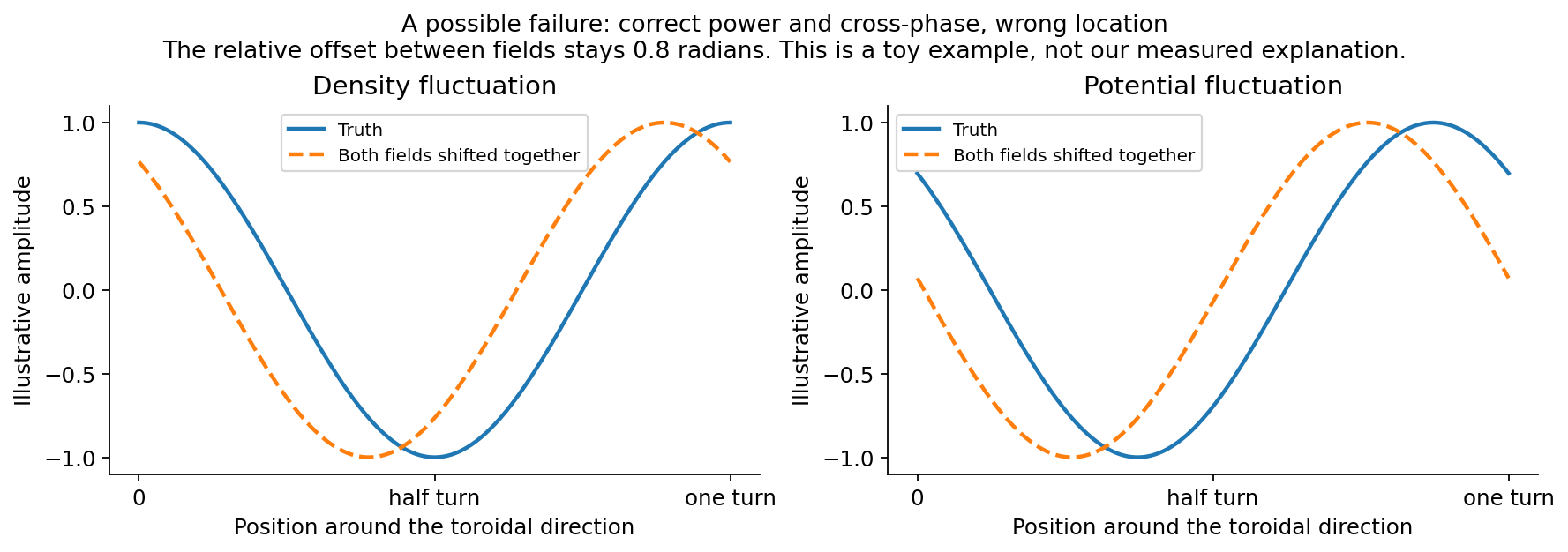
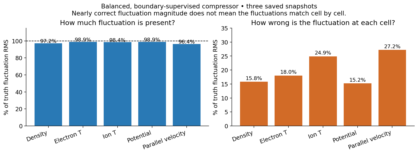
Two different questions: how much fluctuation is present, and whether the model reconstructs the actual fluctuation at the right place. The first can be right while the second is wrong.
Quantity
What it asks
What it does not establish
Fluctuation RMS
How large is q′ = q − instantaneous toroidal mean?
Whether model and truth have the same structures
Power spectrum
How is fluctuation variance distributed across toroidal modes?
Correct phase or position
Cross-phase
How are two fields aligned within a mode?
Alignment of each field with truth; shared shifts can preserve cross-phase
Local cross-phase error
Does the field-pair phase match truth at each location before averaging?
Correct amplitudes or a complete transport budget
Fluctuation RMSE
How different are model q′ and truth q′ at corresponding cells?
By itself, whether amplitude or phase caused that difference
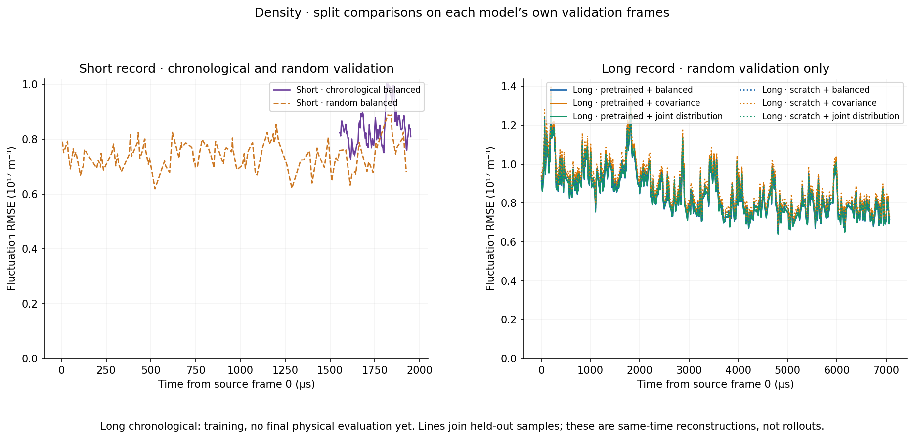
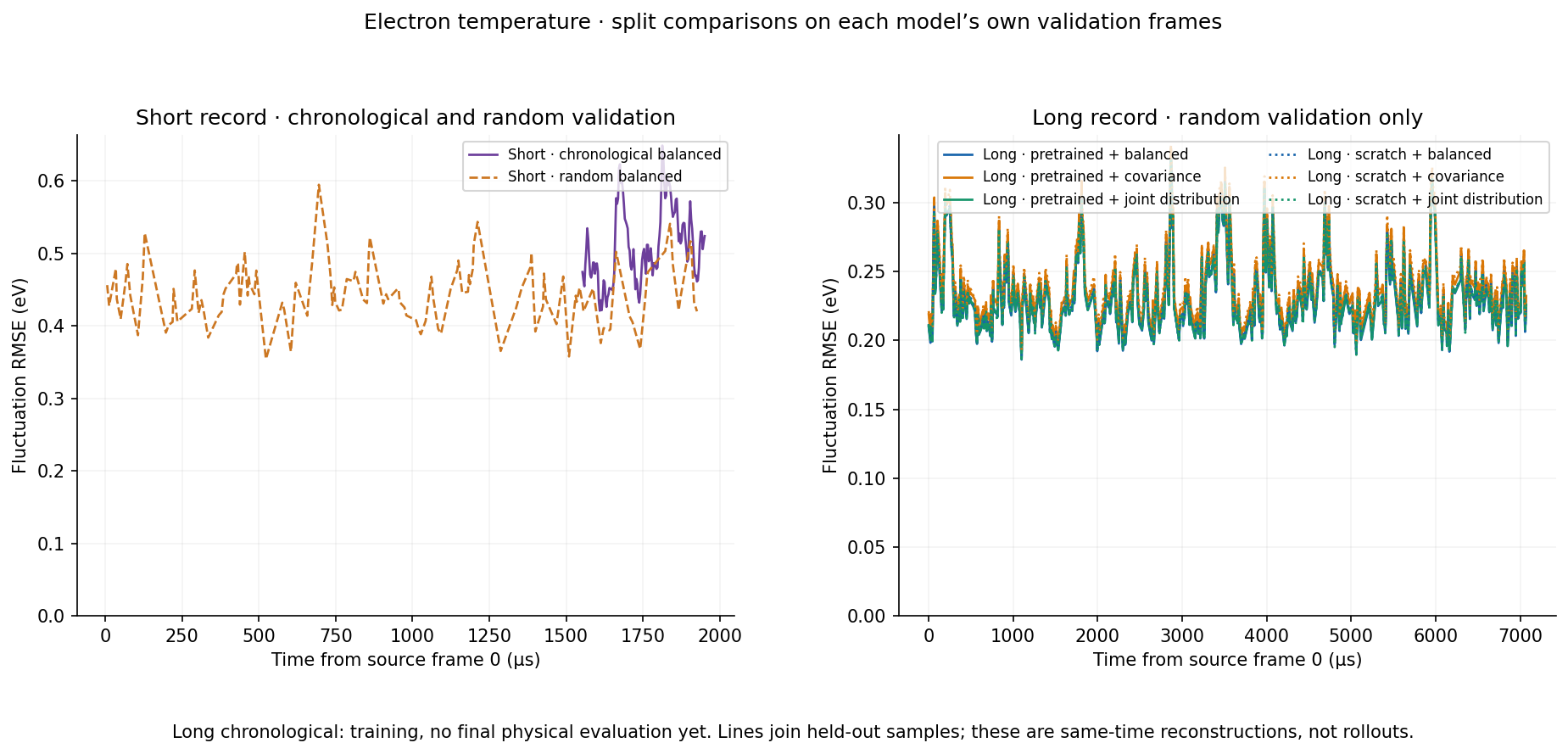
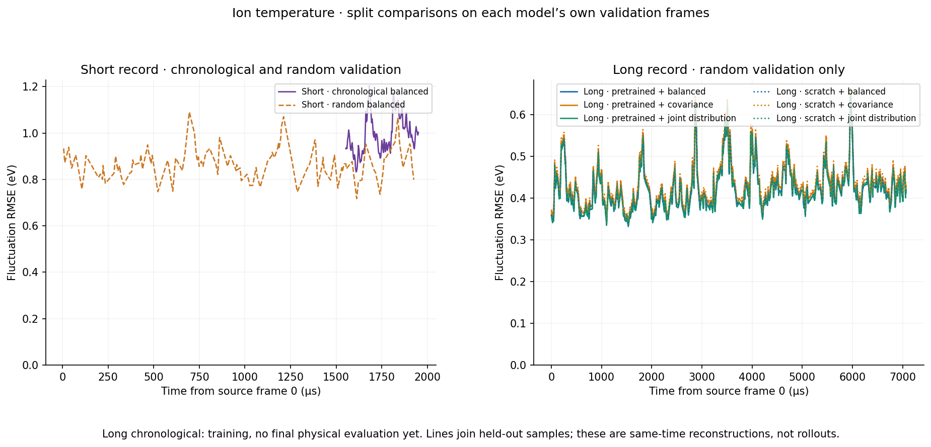
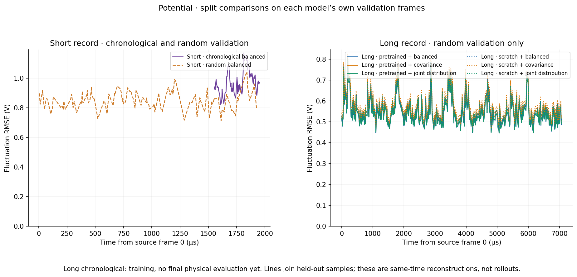
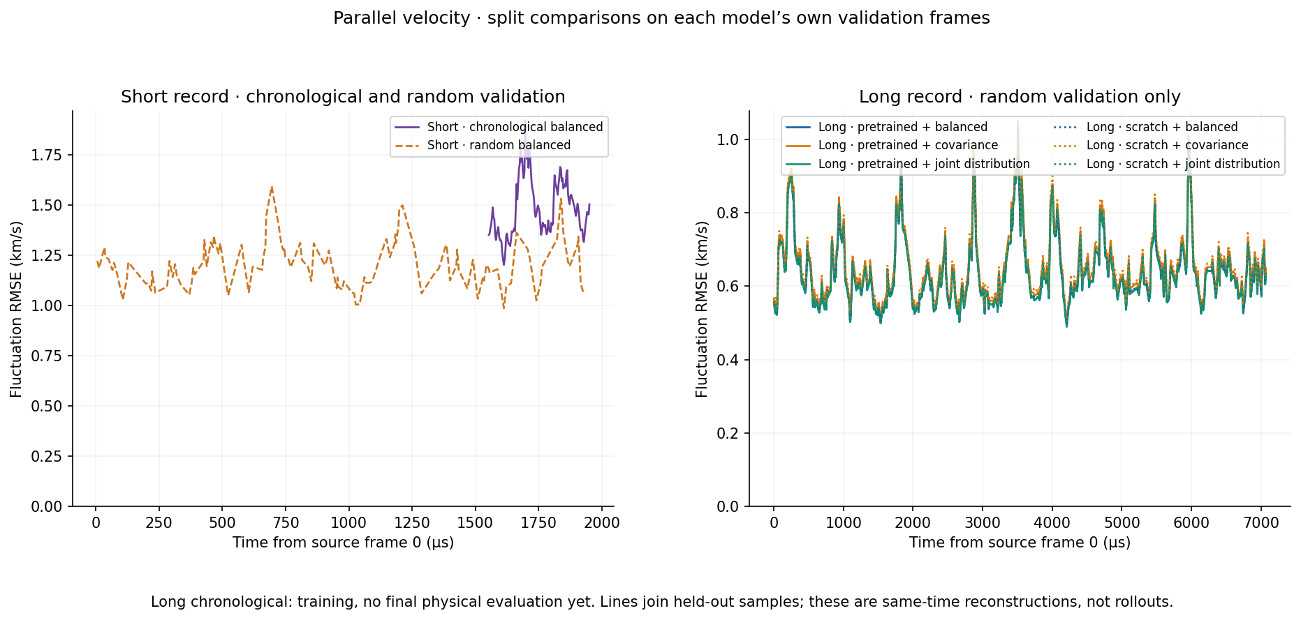
Split comparison · fluctuation-error curves through time
Density · short and long split comparisons. Left: short chronological and short random balanced models, on their respective validation frames. Right: six long random-split models on identical long validation frames. Long chronological final curves remain pending. These are distinct from the short joint-distribution reference in the next gallery. Download
Electron temperature · short and long split comparisons. Left: short chronological and short random balanced models, on their respective validation frames. Right: six long random-split models on identical long validation frames. Long chronological final curves remain pending. These are distinct from the short joint-distribution reference in the next gallery. Download
Ion temperature · short and long split comparisons. Left: short chronological and short random balanced models, on their respective validation frames. Right: six long random-split models on identical long validation frames. Long chronological final curves remain pending. These are distinct from the short joint-distribution reference in the next gallery. Download
Potential · short and long split comparisons. Left: short chronological and short random balanced models, on their respective validation frames. Right: six long random-split models on identical long validation frames. Long chronological final curves remain pending. These are distinct from the short joint-distribution reference in the next gallery. Download
Parallel velocity · short and long split comparisons. Left: short chronological and short random balanced models, on their respective validation frames. Right: six long random-split models on identical long validation frames. Long chronological final curves remain pending. These are distinct from the short joint-distribution reference in the next gallery. Download
Fluctuation magnitude versus actual reconstruction error. Earlier diagnostic establishing why similar spectra were not sufficient evidence. Download
Local versus pooled errors. Averaging cross-spectra first can hide opposing local phase errors. Download
Fluctuation reconstruction error · line plots
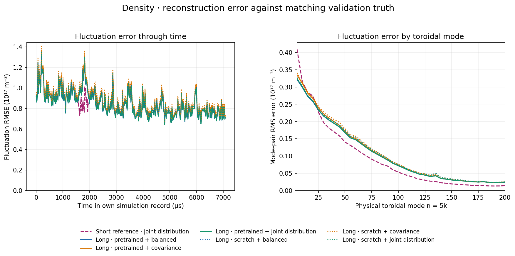
Density · fluctuation error through time and by mode. Short reference evaluated on short-data validation; long models evaluated on long-data validation. Each error uses its own matching truth. Left: spatial RMSE at each held-out frame, not a rollout. Right: RMS contribution of each nonzero conjugate mode pair; squared contributions sum to total fluctuation MSE. Different source records are not a controlled data-size comparison. Download
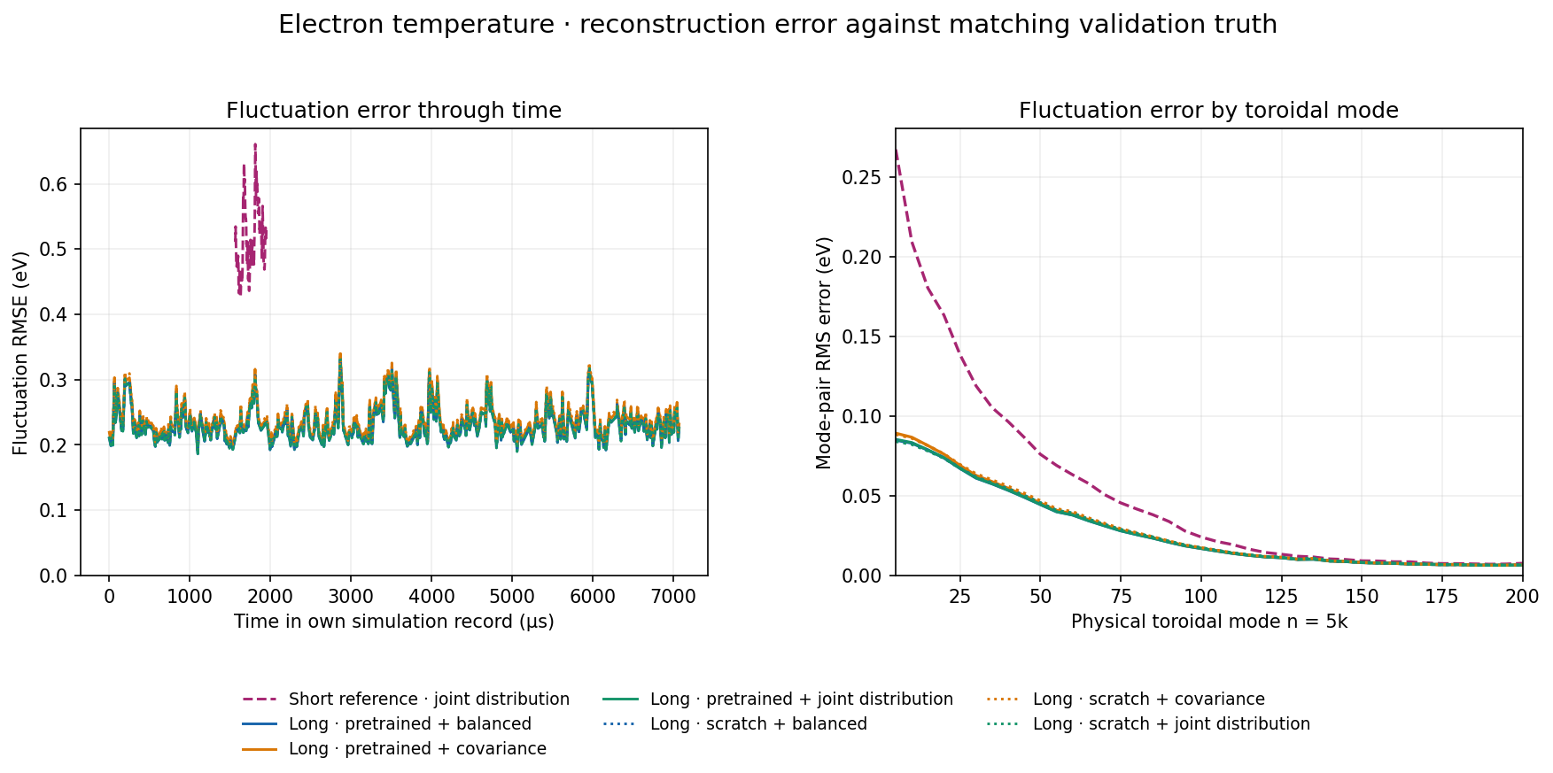
Electron temperature · fluctuation error through time and by mode. Short reference evaluated on short-data validation; long models evaluated on long-data validation. Each error uses its own matching truth. Left: spatial RMSE at each held-out frame, not a rollout. Right: RMS contribution of each nonzero conjugate mode pair; squared contributions sum to total fluctuation MSE. Different source records are not a controlled data-size comparison. Download
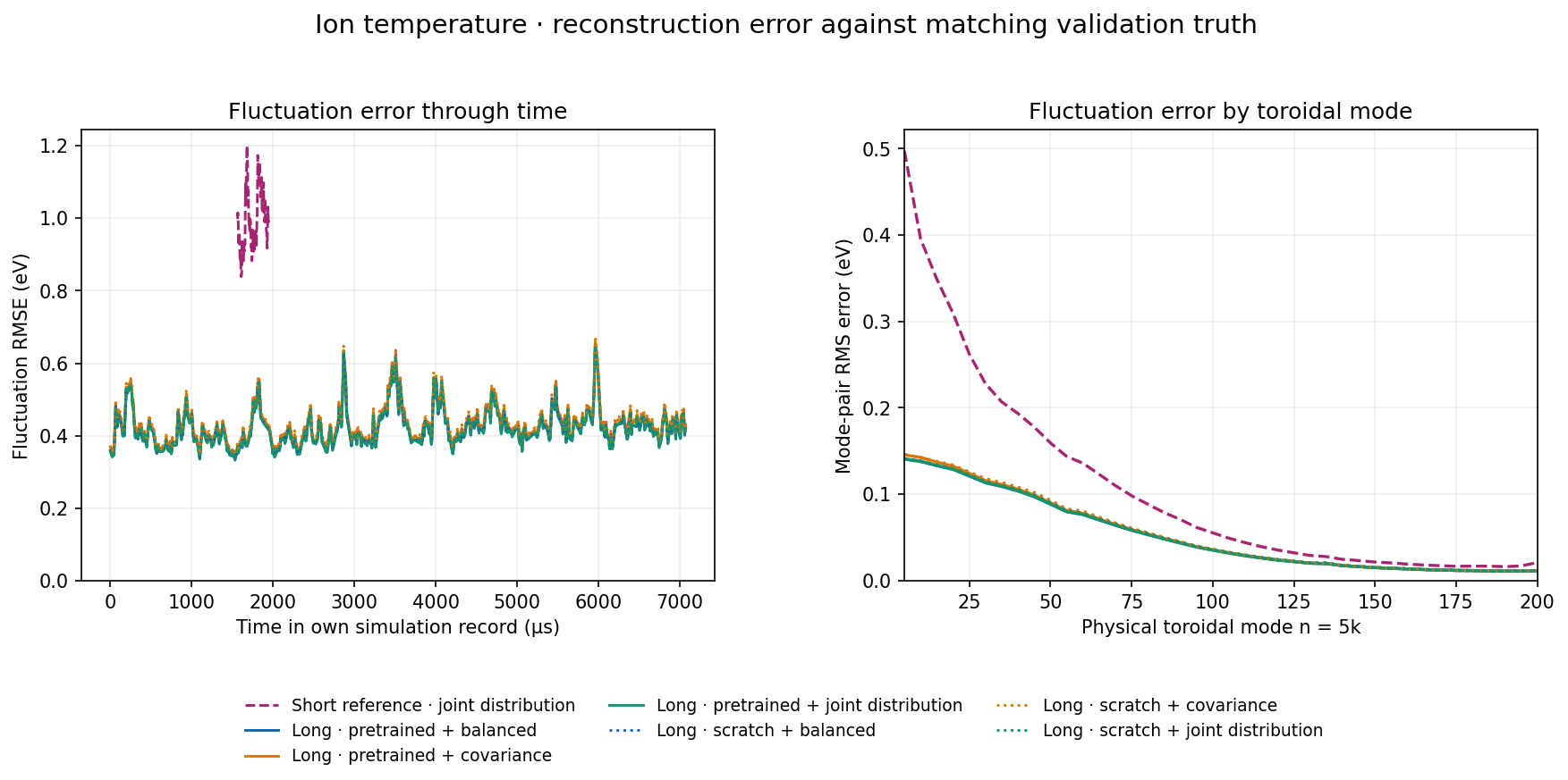
Ion temperature · fluctuation error through time and by mode. Short reference evaluated on short-data validation; long models evaluated on long-data validation. Each error uses its own matching truth. Left: spatial RMSE at each held-out frame, not a rollout. Right: RMS contribution of each nonzero conjugate mode pair; squared contributions sum to total fluctuation MSE. Different source records are not a controlled data-size comparison. Download
Potential · fluctuation error through time and by mode. Short reference evaluated on short-data validation; long models evaluated on long-data validation. Each error uses its own matching truth. Left: spatial RMSE at each held-out frame, not a rollout. Right: RMS contribution of each nonzero conjugate mode pair; squared contributions sum to total fluctuation MSE. Different source records are not a controlled data-size comparison. Download
Parallel velocity · fluctuation error through time and by mode. Short reference evaluated on short-data validation; long models evaluated on long-data validation. Each error uses its own matching truth. Left: spatial RMSE at each held-out frame, not a rollout. Right: RMS contribution of each nonzero conjugate mode pair; squared contributions sum to total fluctuation MSE. Different source records are not a controlled data-size comparison. Download
Resolution: the earlier spectrum plots were useful amplitude diagnostics, but we overinterpreted them as evidence of local reconstruction fidelity. Keep amplitude, complex error, local cross-phase and transport together. Better pooled phase alone is not a demonstrated fix.
3. Diffusion: what we changed, and what it helped
Four true history volumes→Frozen short-data encoder→Conditional diffusion predicts next latent→Frozen decoder→Predicted volume; feed latent back
Completed model
Conditioning / target
Change tested
History only
Four history latents → full future latent
No deterministic forecast context
Forecast conditioned
History + frozen deterministic forecast → full future latent
Extra conditioning; still not residual diffusion
Forecast + physical loss
Same as forecast conditioned
Decoded physical auxiliary loss, weight 0.1 at low noise
Forecast + history-noise curriculum
Same full target, progressively corrupted history
Noise cap grows to 0.35 over first 4,096 updates; 50% clean history
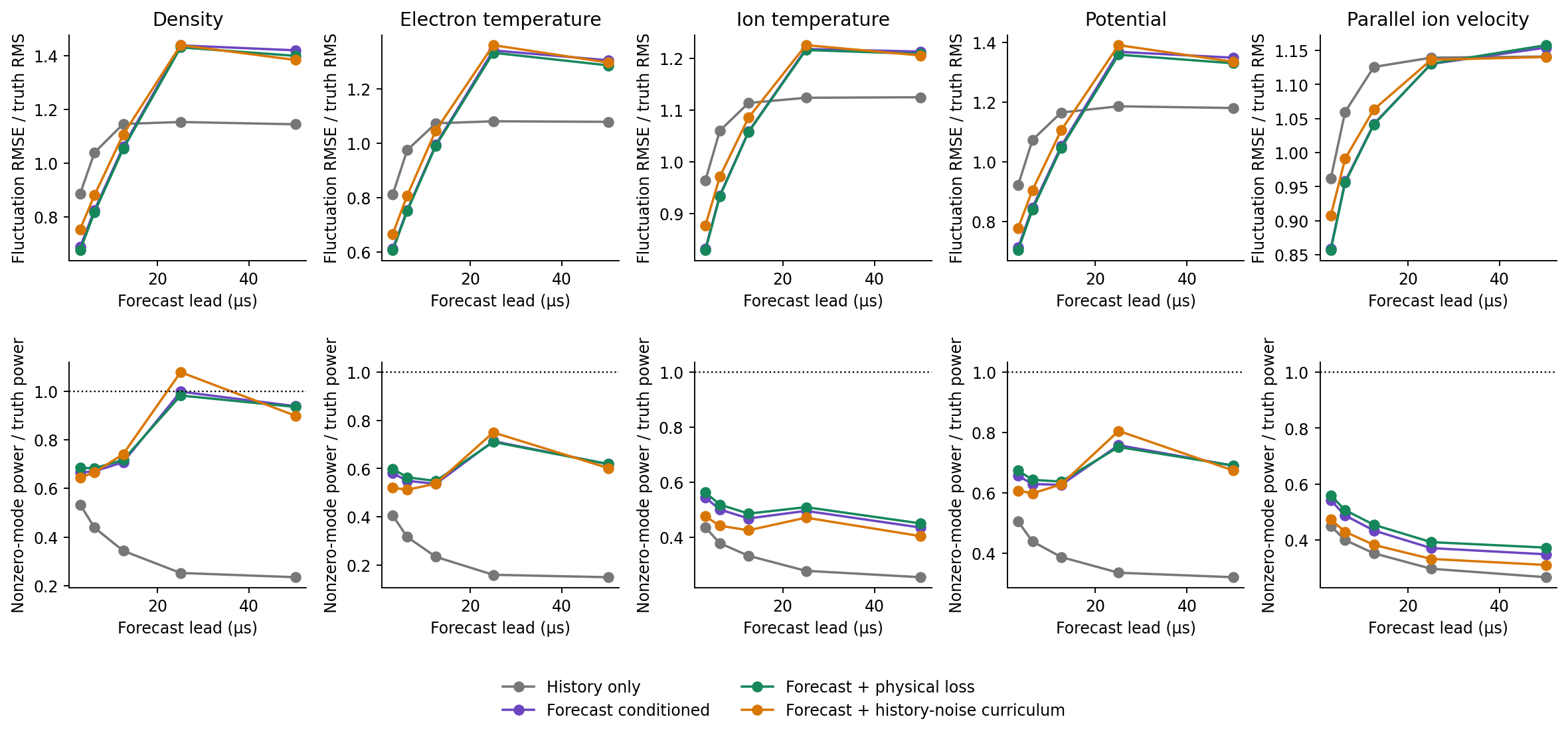
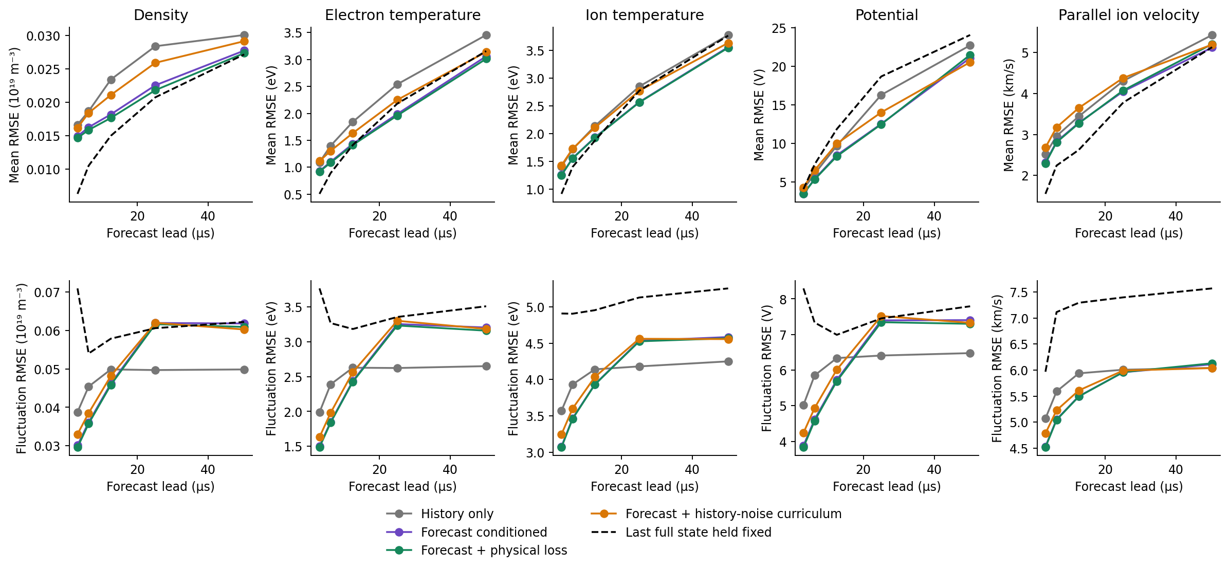
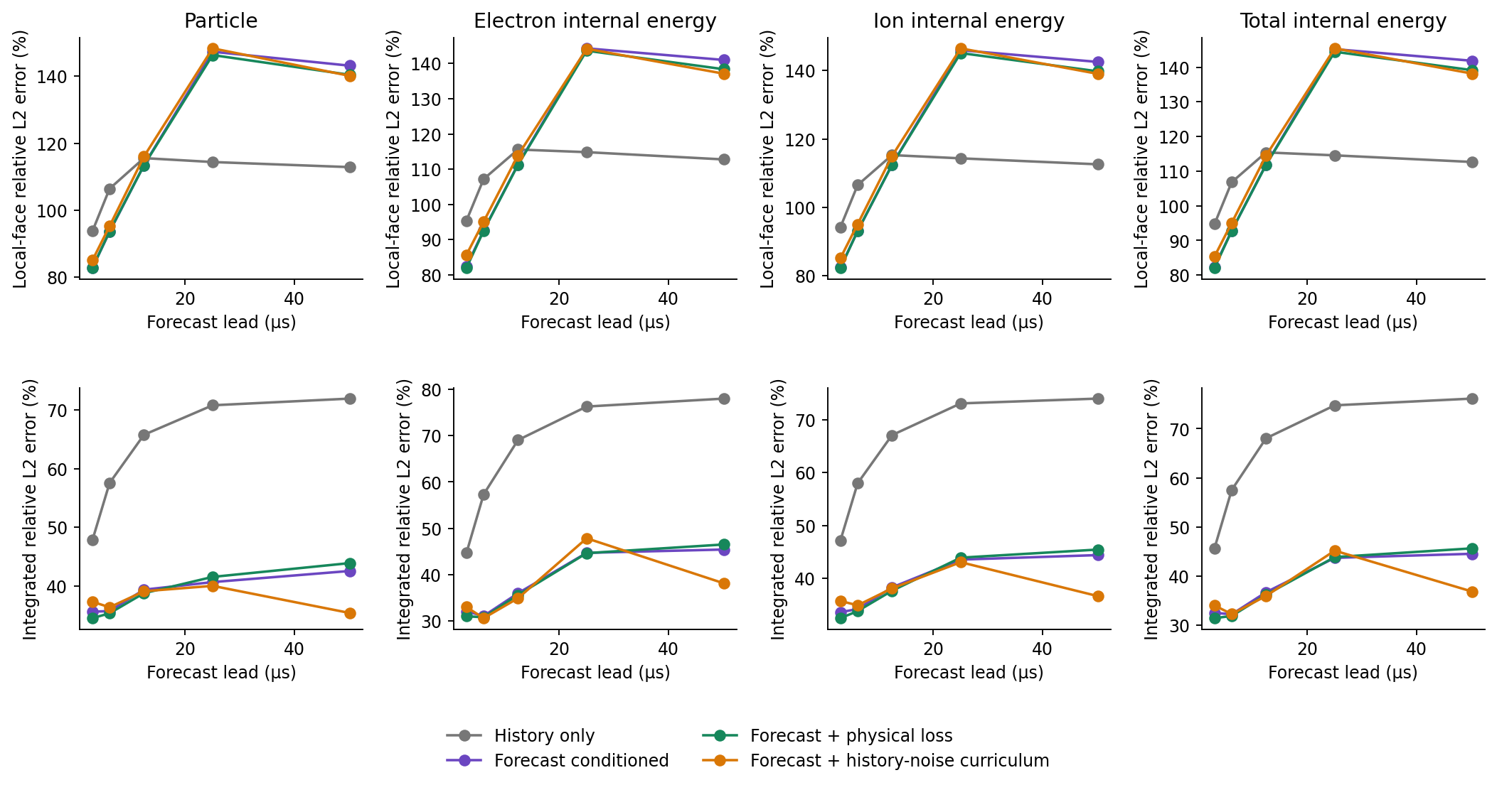
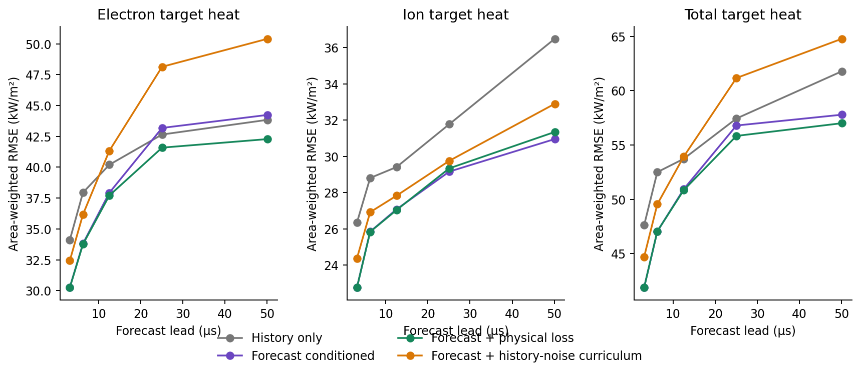
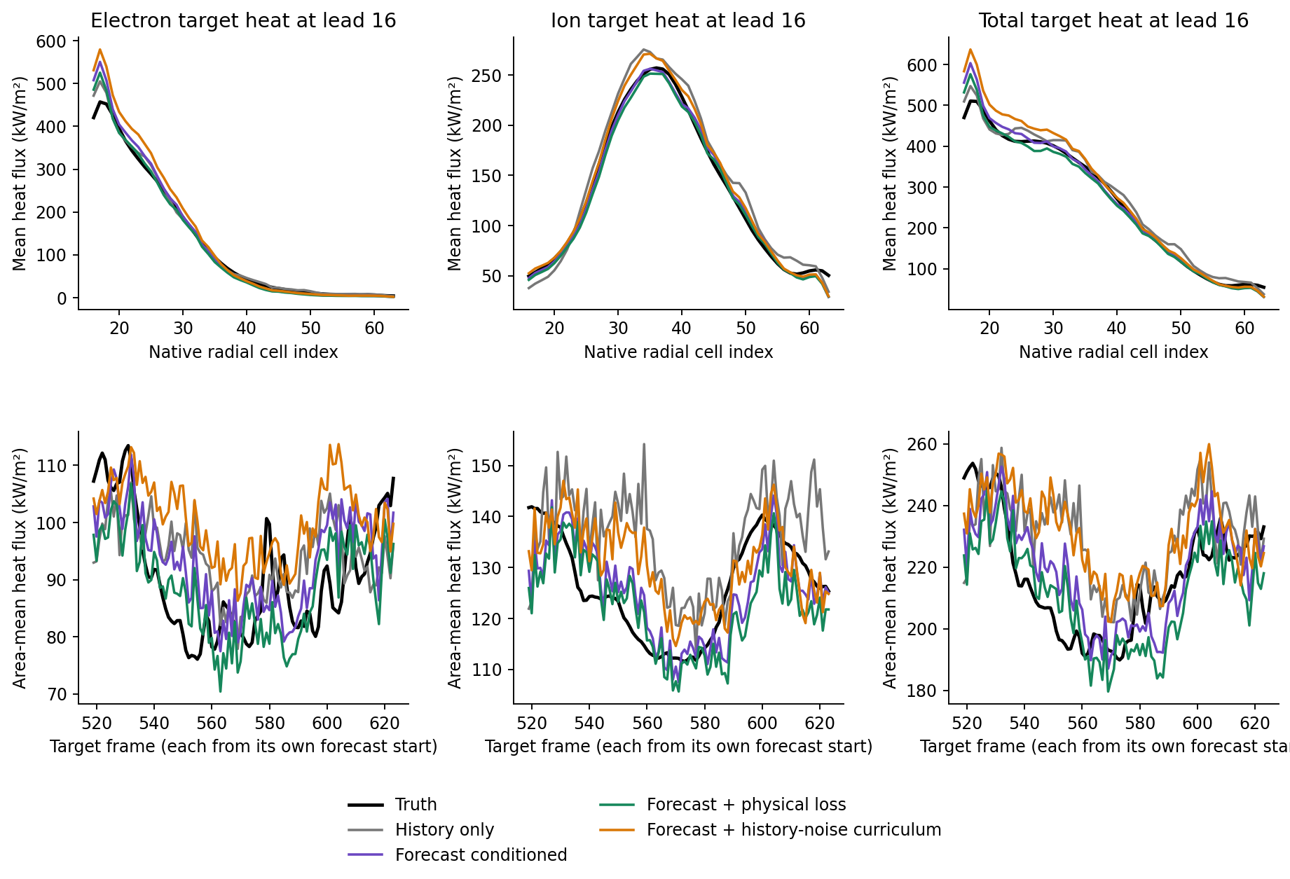
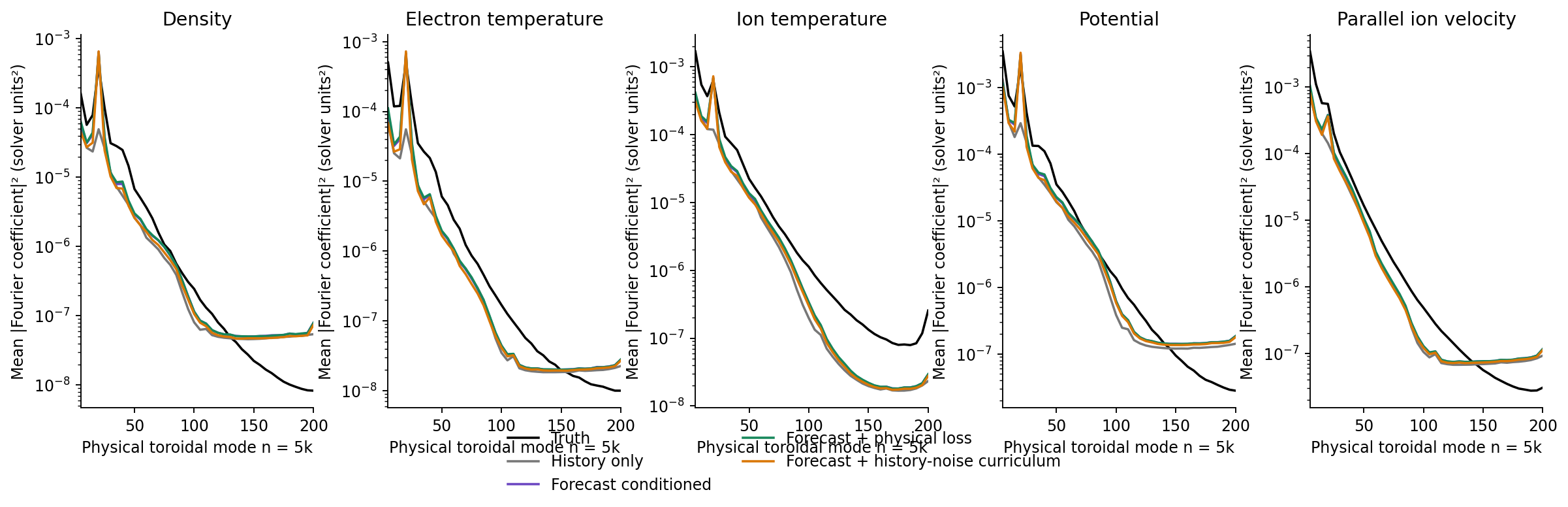
Four fresh seed-0 denoisers, 16,384 updates each, same frozen short-data codec; 32 DDIM sampling steps. Evaluation: 105 overlapping chronological validation starts, one sampled path per start, leads 1–16 (about 3.13–50.11 µs). These are not ensemble-calibration results. The physical-loss and history-noise arms are separate changes to the forecast-conditioned control.
Forecast performance through time
Fluctuation error and amplitude. Pointwise error and power must be read together; amplitude restoration is not trajectory recovery. Download
All five physical fields. Errors versus forecast lead, not same-time reconstruction. Download
Particle and energy transport. Radial transport errors, distinct from target sheath heat. Download
Electron, ion and total target-heat errors. Recovered target estimates versus forecast lead. Download
Target heat: truth and forecast. Shows profile shape as well as aggregate error. Download
Forecast toroidal spectra. Full available modes; correct power does not require correct phase. Download
Pooled cross-phase at lead 1. Pooled statistic only, not a local cross-phase error test. Download
Pooled cross-phase at lead 16. Do not equate this with spatially correct turbulent structure. Download
Forecast conditioning improved the first-step result and retained more power. History noise reduced integrated particle error but worsened target-heat error relative to clean forecast conditioning. No one recipe wins every observable. The new long-data and block/rolling tests have not yet produced results.
Earlier temporal ablations: what these builds on
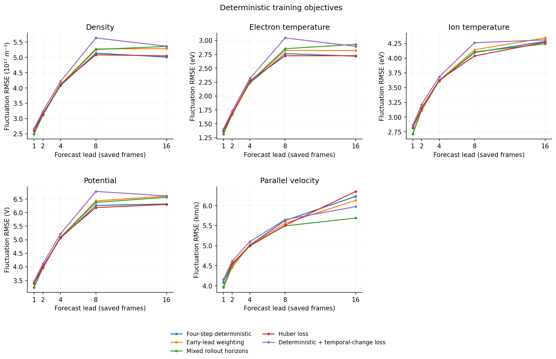
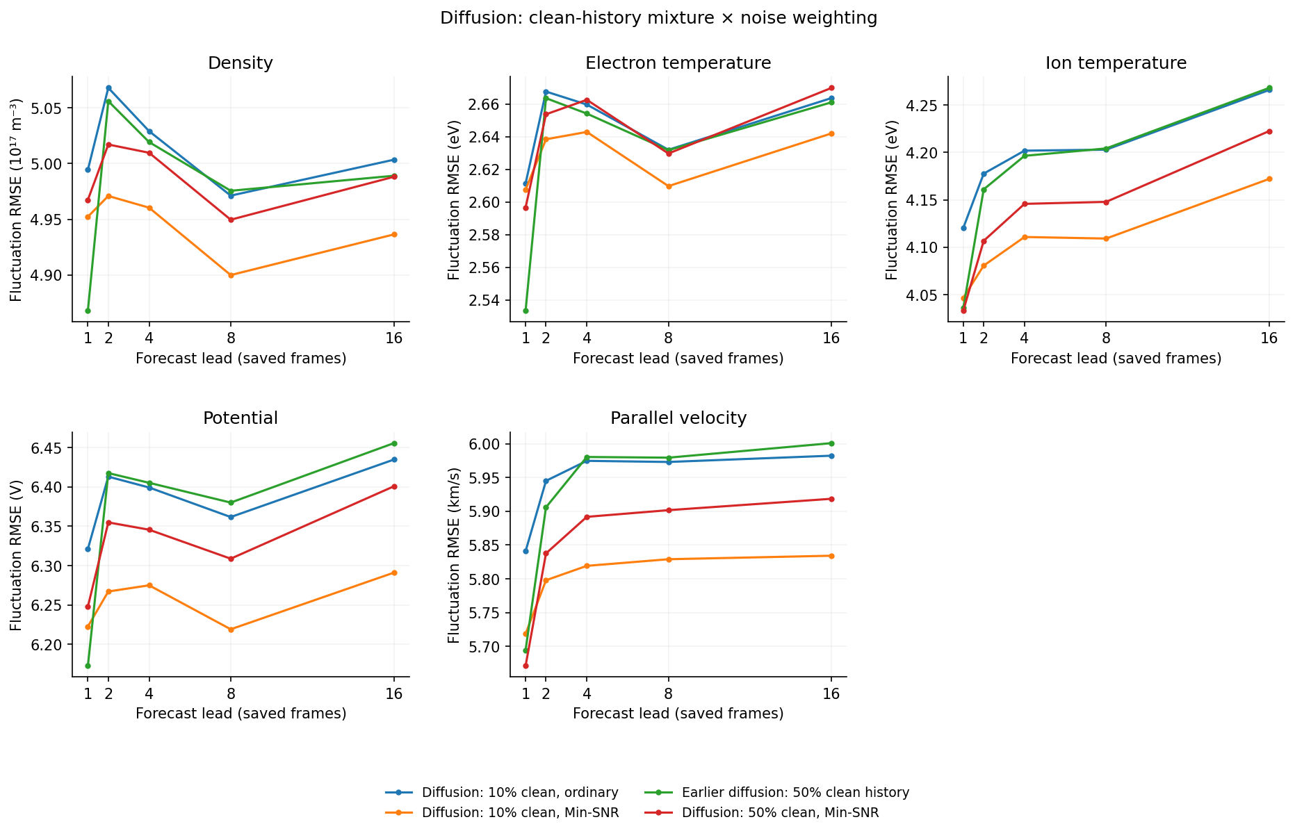
Earlier families
Deterministic training objectives. Earlier controls; see original report for each training budget. Download
Diffusion history mixture and noise weighting. Earlier recipe comparison; not the new long-data models. Download
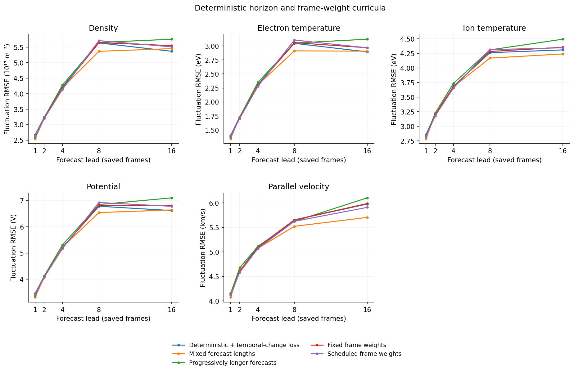
Horizon and frame-weight curricula. Changes which forecast horizons training emphasizes. Download
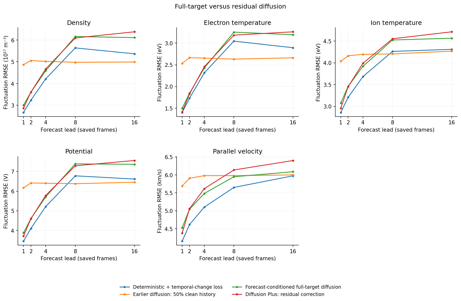
Full-target versus residual diffusion. Residual predicts a correction to a forecast; full-target predicts the future latent itself. Download
Long-data random-split balanced compressor→Independent 85606 fine-tune: 6,400 updates→Train both encoder and decoder→Same held-out 128 target-shot frames
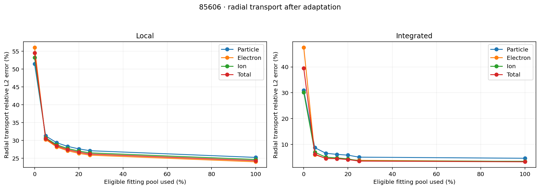
Fractions 5/10/15/20/25/100% use 22/43/65/86/108/432 eligible fitting frames. 0% is the unadapted model. All use the same evaluation frames [496,624); 100% does not include guard or validation frames. Each fraction starts from the same parent rather than continuing the previous fraction. Balanced reconstruction objective; no old-shot replay in these runs.
Completed long-parent fraction sweep
All five fluctuation errors. All six fine-tunes completed. More target data continues reducing each field error. Download
Local and integrated radial transport. Electron/ion energy transport is not 85606 target sheath heat; the latter is unavailable in this evaluator. Download
Earlier comparisons and retained source skill
Short versus long parent. Earlier figure includes only fractions available when generated; the complete long-parent sweep is immediately above. Download
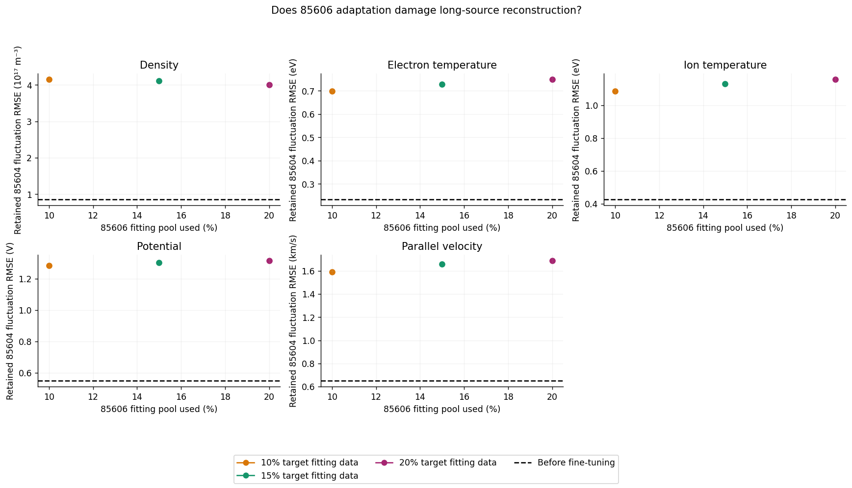
Retained long-source reconstruction. Earlier partial-coverage retention view; do not infer missing fractions. Download
There is no demonstrated fraction where all metrics saturate: 25% remains worse than 100% on all five fluctuation errors. The 85606 record has now been used for adaptation and repeated development evaluation; it is not a fresh blind shot test.
5. Can a tiny XY input match full-XZ input at the divertor?
This is the actual observation goal. “Full XZ” describes the OMP input slab. The output of interest is a different XZ plane at the outer divertor.
Training: five fields on the downstream region x16–63, y20–31, including target y31; normalized mean/fluctuation GradNorm with clean reconstruction replay coefficient 0.5. AdamW 10⁻⁵ with 100-update warmup, 30,000 updates per adaptation stage. Fit [0,432); evaluate [500,624). Clean replay bypasses the observation adapter. These all use the short-data codec.
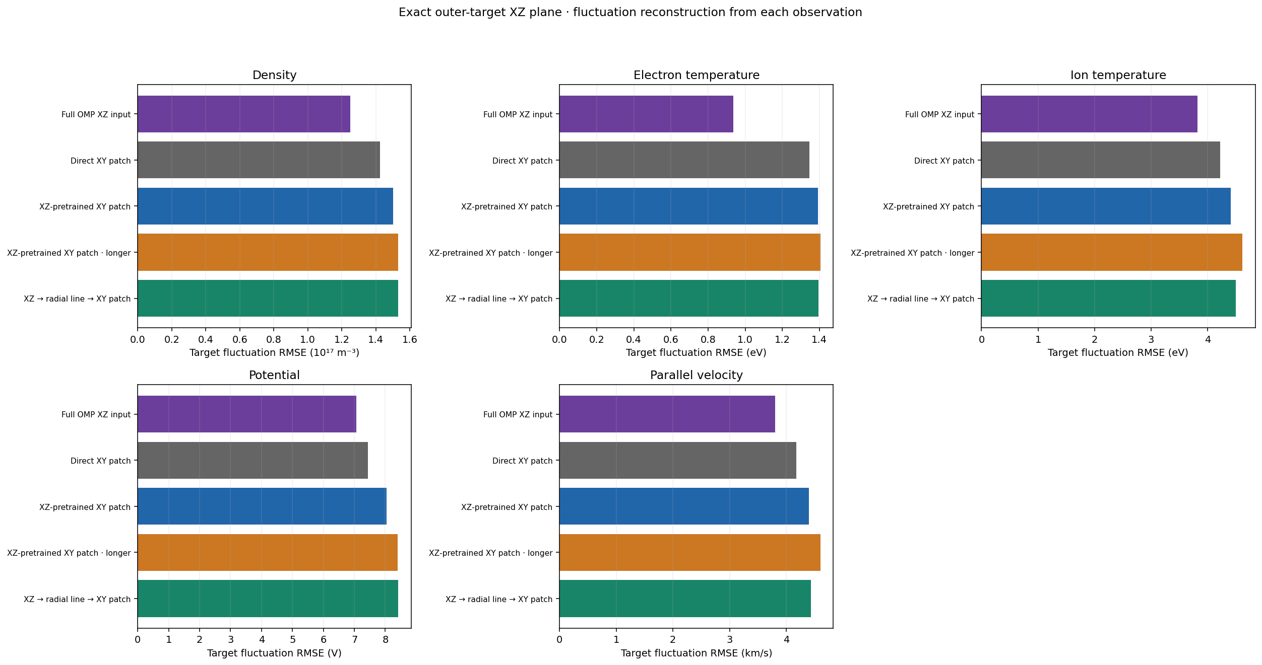
Evaluation: target-only XZ = x16–63, y31, all 81 toroidal positions. Broader downstream-volume scores are separate. We have not tested a target-only training objective in this batch.
Read the lines: one model key for every target plot
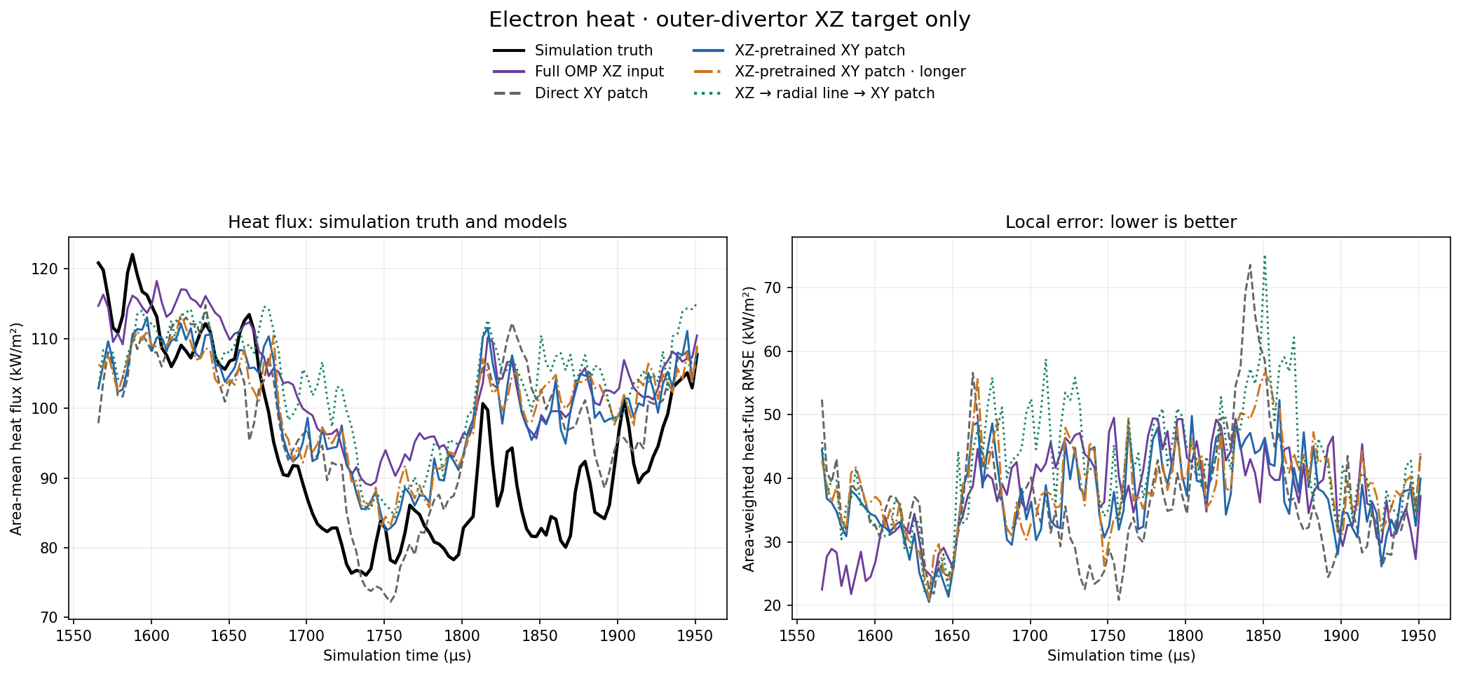
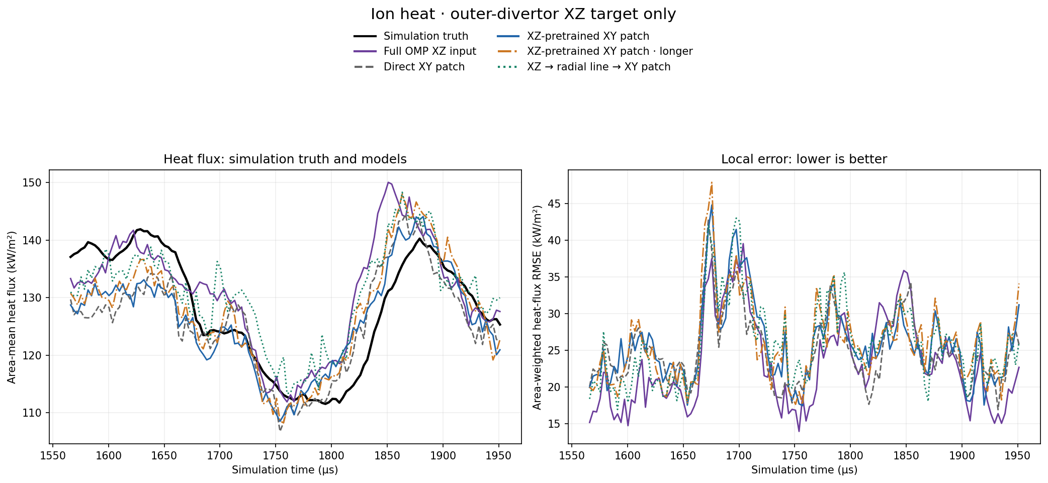
Black = simulation truth. Model colors and line styles below are identical in the heat, power-spectrum and local cross-phase figures. Electron / ion / total identify the physical quantity, not different models.
XZ → radial line → XY patch Same full-OMP-XZ parent → 30k native-radial-line updates → 30k physical-patch updates
Electron heat is the recovered electron contribution at the target; ion heat is the recovered ion contribution; total heat = electron + ion, summed before computing the error. Left panel: area-mean truth/model heat flux. Right panel: local error before area averaging; lower is better. Both use the exact outer-divertor target and common finite support.
Target heat · electron, ion and total
Electron target heat. Exact outer-divertor XZ, x16–63,y31,all toroidal samples; common validation frames500–623. Separate same-time inferences, not time rollouts. Same recovered sheath operator for truth and all models. Download
Ion target heat. Exact outer-divertor XZ, x16–63,y31,all toroidal samples; common validation frames500–623. Separate same-time inferences, not time rollouts. Same recovered sheath operator for truth and all models. Download
Total target heat. Exact outer-divertor XZ, x16–63,y31,all toroidal samples; common validation frames500–623. Separate same-time inferences, not time rollouts. Same recovered sheath operator for truth and all models. Download
Target field errors
Outer-divertor fluctuation errors, all five fields. Same target-only truth and124validation frames for every model. Both ±k Fourier contributions included. Download
Downstream region versus the target: why the earlier curves looked better
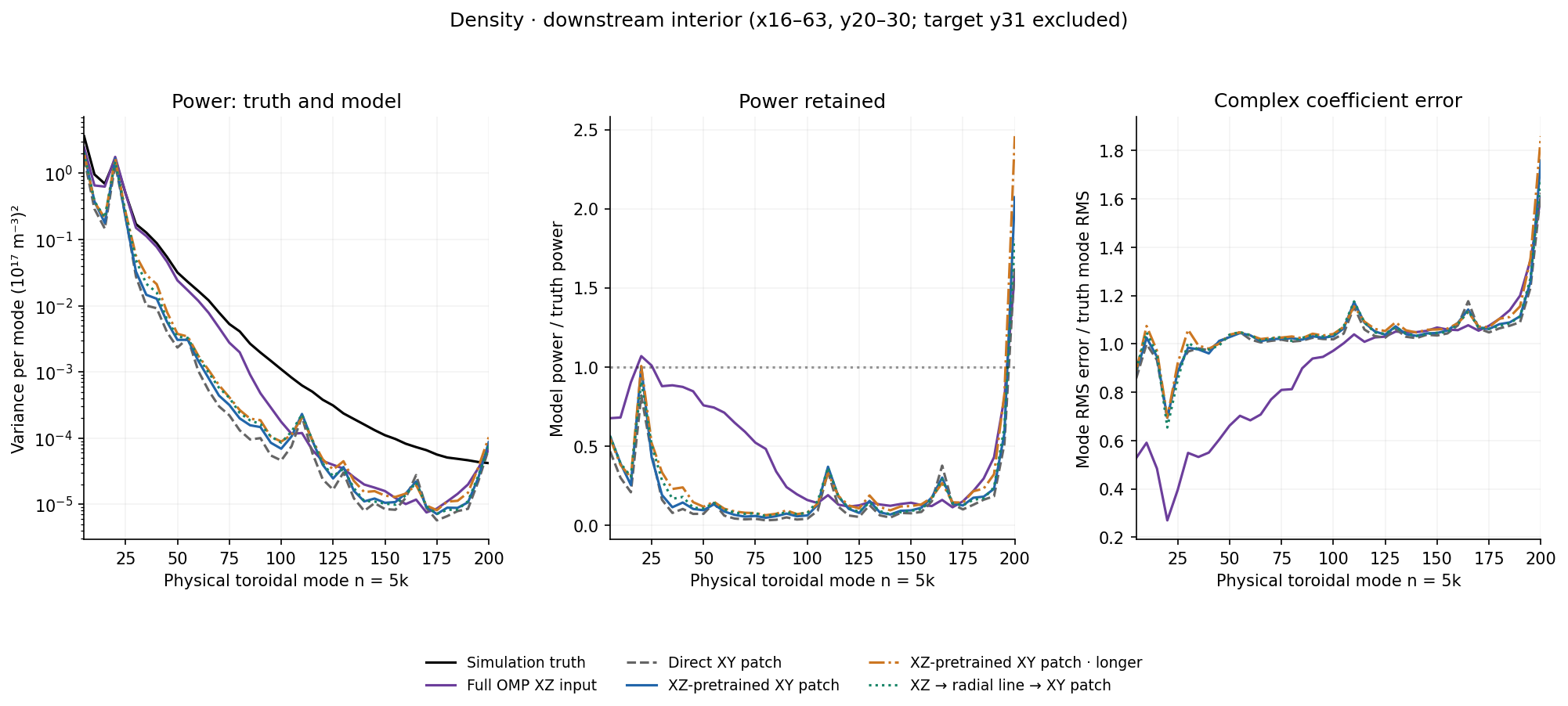
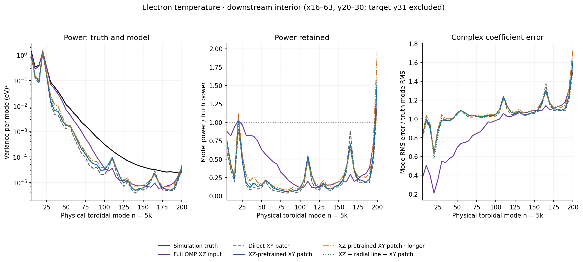
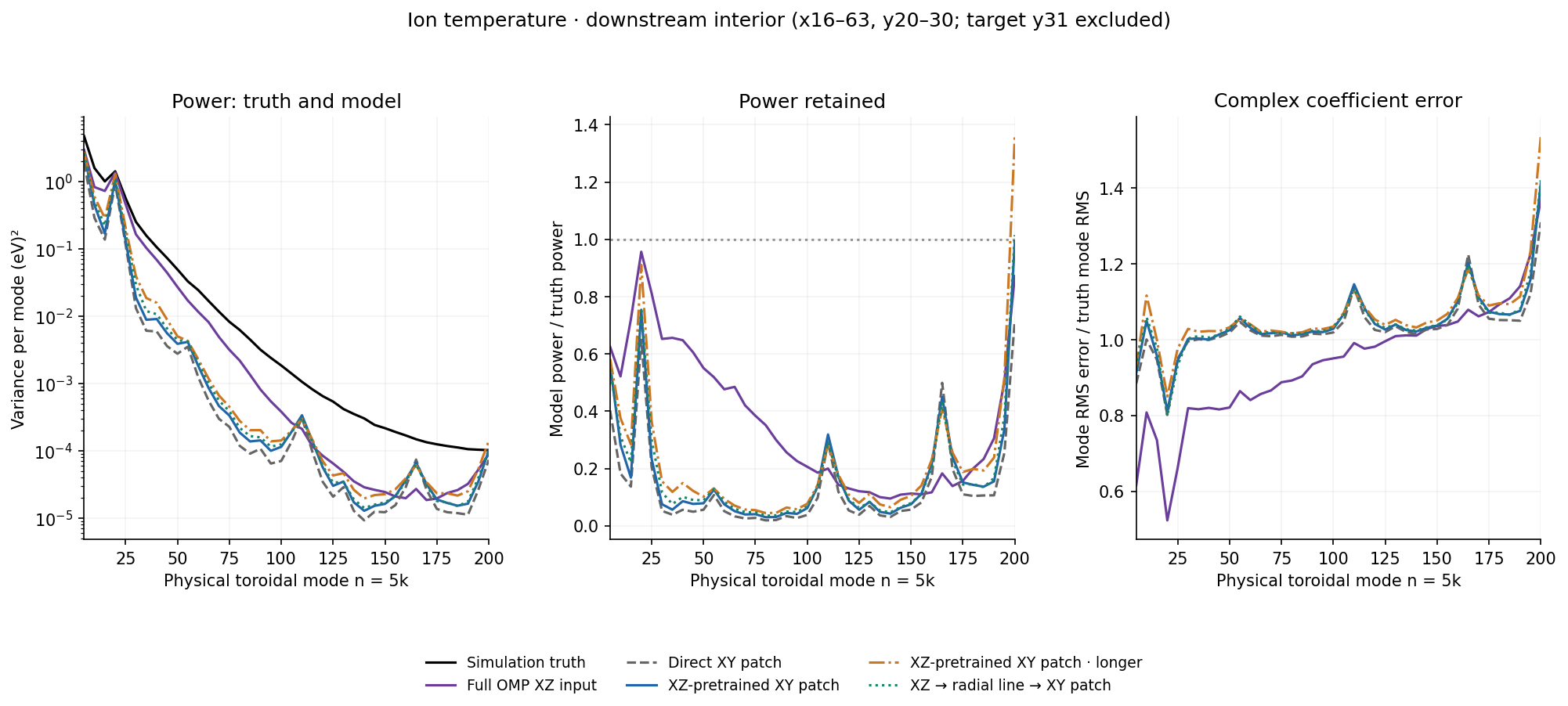
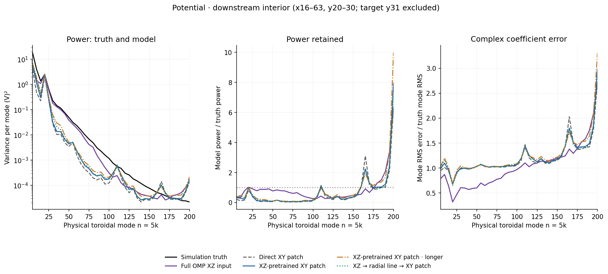
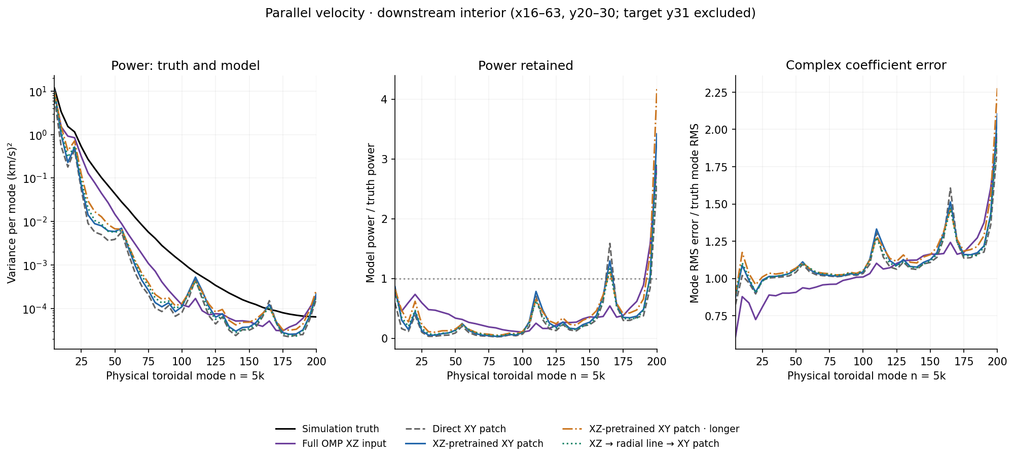
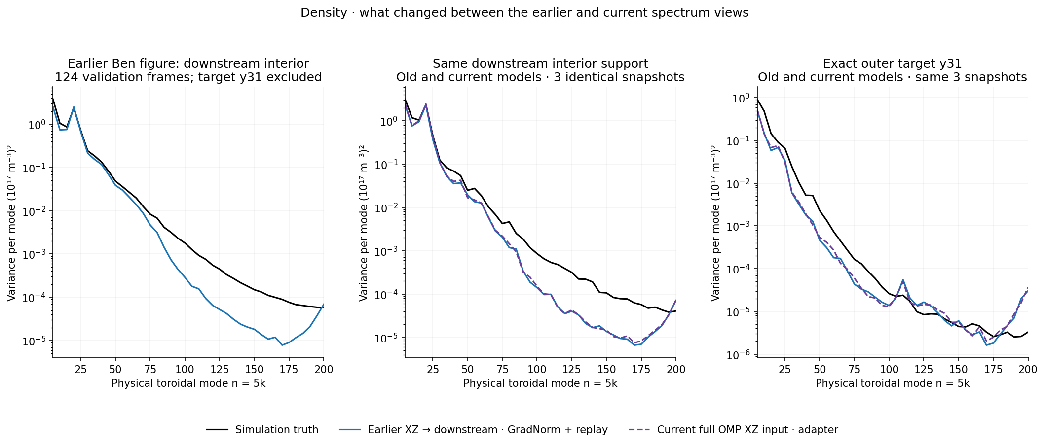
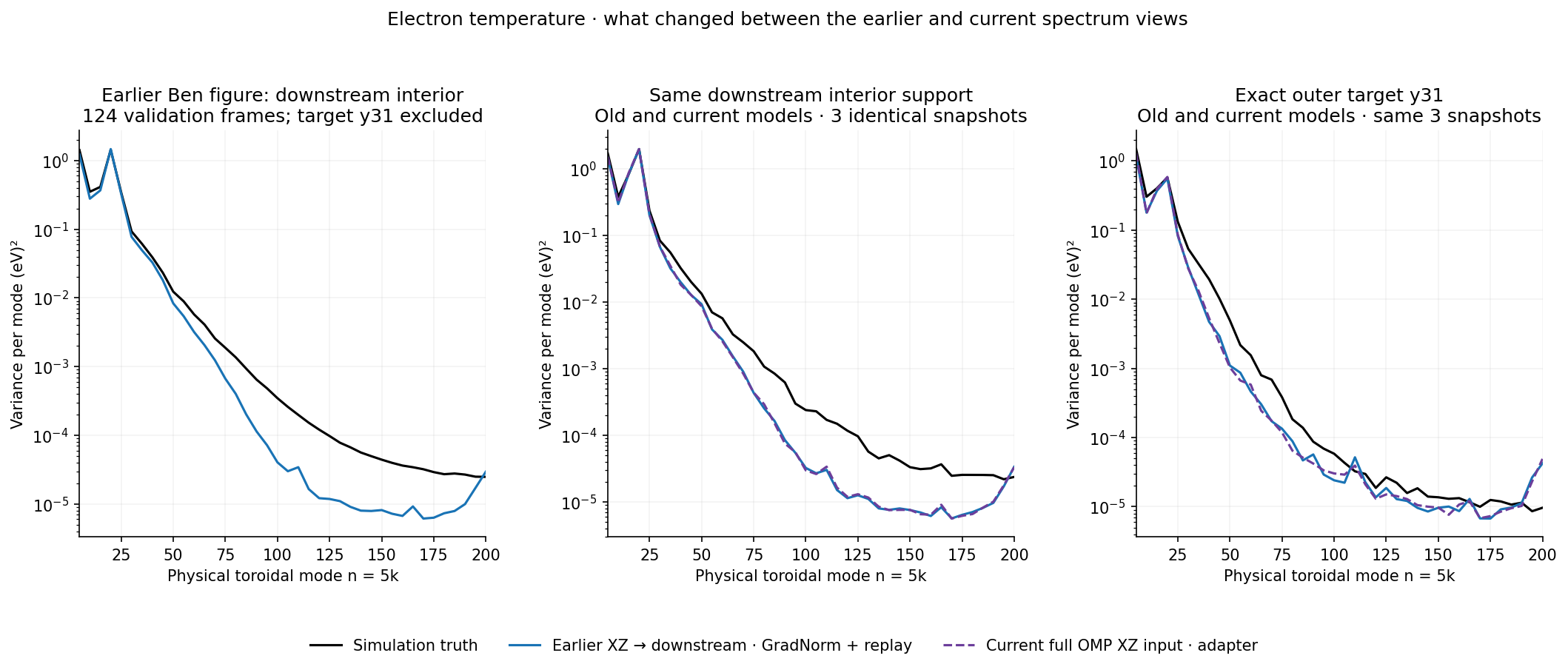
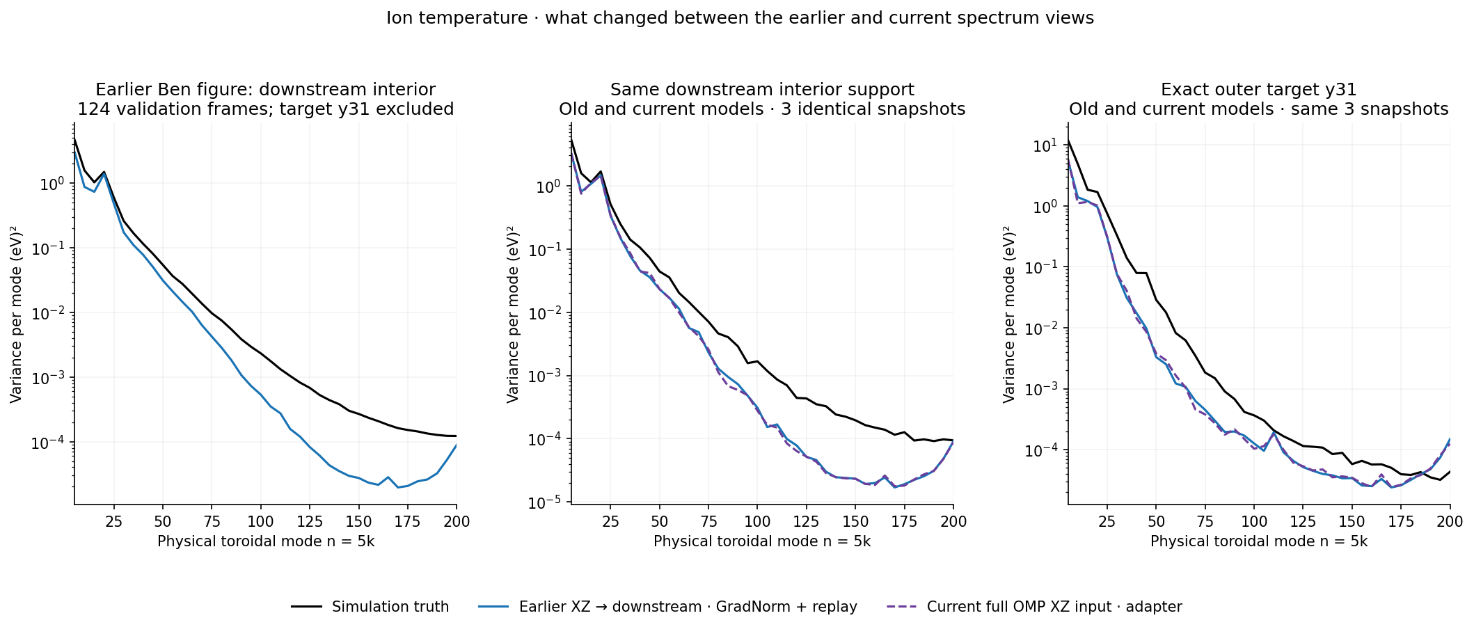
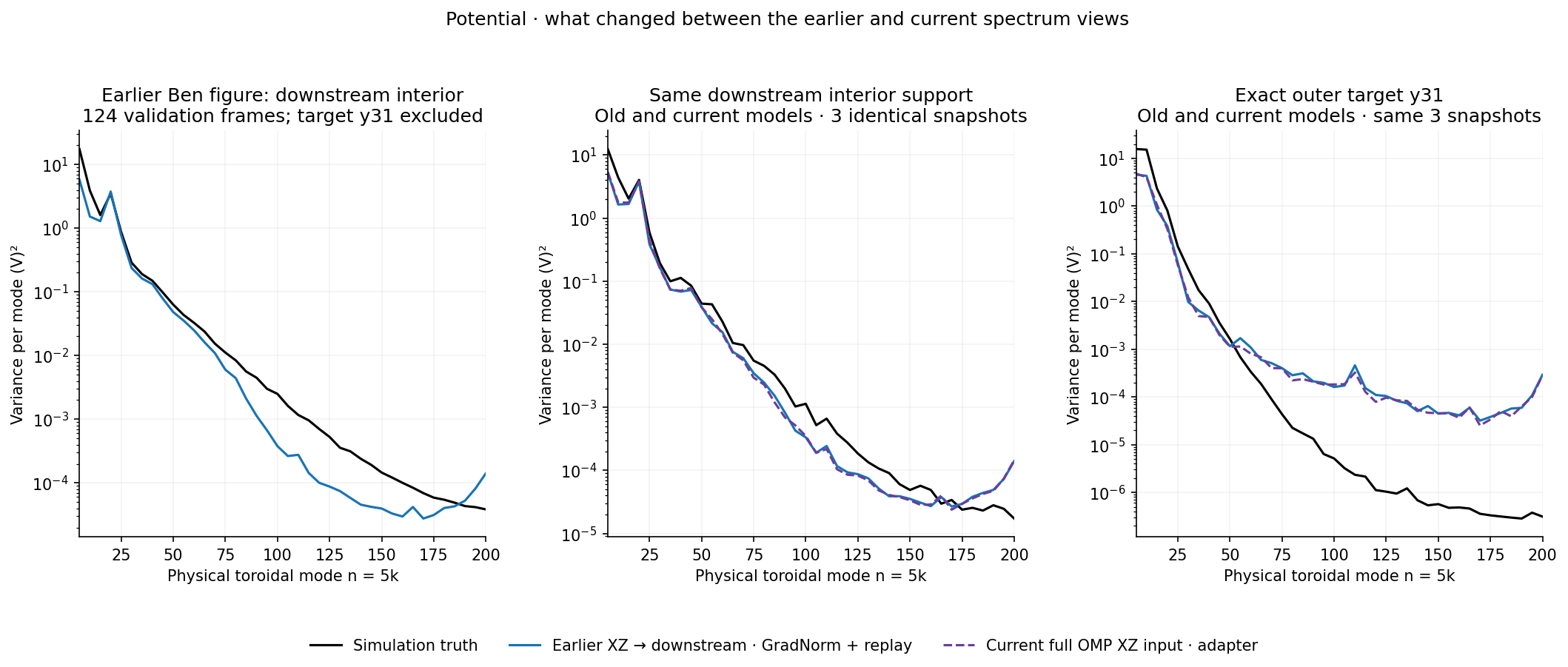
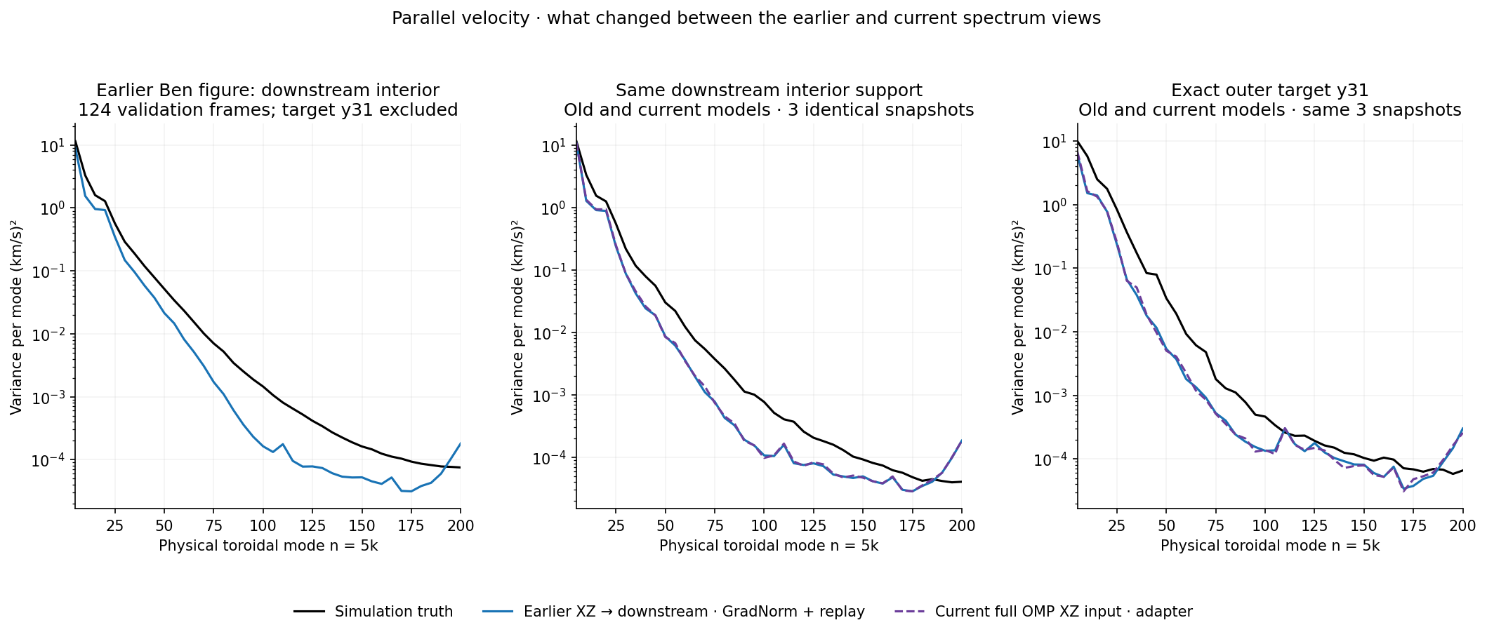
The spectra in the page linked to Ben on October 14 averaged the downstream interior and excluded the boundary y31. The exact-target figures below score y31 alone. “Downstream region” and “outer-divertor target” are therefore separate choices, not interchangeable labels. The earlier model also used direct masked-volume input, whereas the current full-XZ control uses a trainable observation adapter.
Current models · downstream-region spectra
Density · downstream interior spectra. All five current models on the same 124 validation frames and interior support x16–63,y20–30 with native masks. Target y31 excluded. Same model names/colors as target-only plots. Download
Electron temperature · downstream interior spectra. All five current models on the same 124 validation frames and interior support x16–63,y20–30 with native masks. Target y31 excluded. Same model names/colors as target-only plots. Download
Ion temperature · downstream interior spectra. All five current models on the same 124 validation frames and interior support x16–63,y20–30 with native masks. Target y31 excluded. Same model names/colors as target-only plots. Download
Potential · downstream interior spectra. All five current models on the same 124 validation frames and interior support x16–63,y20–30 with native masks. Target y31 excluded. Same model names/colors as target-only plots. Download
Parallel velocity · downstream interior spectra. All five current models on the same 124 validation frames and interior support x16–63,y20–30 with native masks. Target y31 excluded. Same model names/colors as target-only plots. Download
Earlier Ben reference versus current full-XZ control
Density · earlier view and matched region/target check. Left: earlier 124-frame downstream spectrum shown on the shared page. Middle/right: old and current models on exactly the same three saved snapshots (512,560,623), with identical truth and weights within each panel. Middle is common downstream interior; right is exact target y31. Three snapshots are a diagnostic, not the full spectral evaluation. Download
Electron temperature · earlier view and matched region/target check. Left: earlier 124-frame downstream spectrum shown on the shared page. Middle/right: old and current models on exactly the same three saved snapshots (512,560,623), with identical truth and weights within each panel. Middle is common downstream interior; right is exact target y31. Three snapshots are a diagnostic, not the full spectral evaluation. Download
Ion temperature · earlier view and matched region/target check. Left: earlier 124-frame downstream spectrum shown on the shared page. Middle/right: old and current models on exactly the same three saved snapshots (512,560,623), with identical truth and weights within each panel. Middle is common downstream interior; right is exact target y31. Three snapshots are a diagnostic, not the full spectral evaluation. Download
Potential · earlier view and matched region/target check. Left: earlier 124-frame downstream spectrum shown on the shared page. Middle/right: old and current models on exactly the same three saved snapshots (512,560,623), with identical truth and weights within each panel. Middle is common downstream interior; right is exact target y31. Three snapshots are a diagnostic, not the full spectral evaluation. Download
Parallel velocity · earlier view and matched region/target check. Left: earlier 124-frame downstream spectrum shown on the shared page. Middle/right: old and current models on exactly the same three saved snapshots (512,560,623), with identical truth and weights within each panel. Middle is common downstream interior; right is exact target y31. Three snapshots are a diagnostic, not the full spectral evaluation. Download
Same-target check over all 124 frames: current full-XZ fluctuation RMSE differs from the earlier adaptive+replay model by −1.14% density, −0.08% electron temperature, −1.06% ion temperature, −1.92% potential and −0.93% parallel velocity. This is near-parity, not a target collapse. Both can still have substantial target error. Checkpoint-result and support audit.
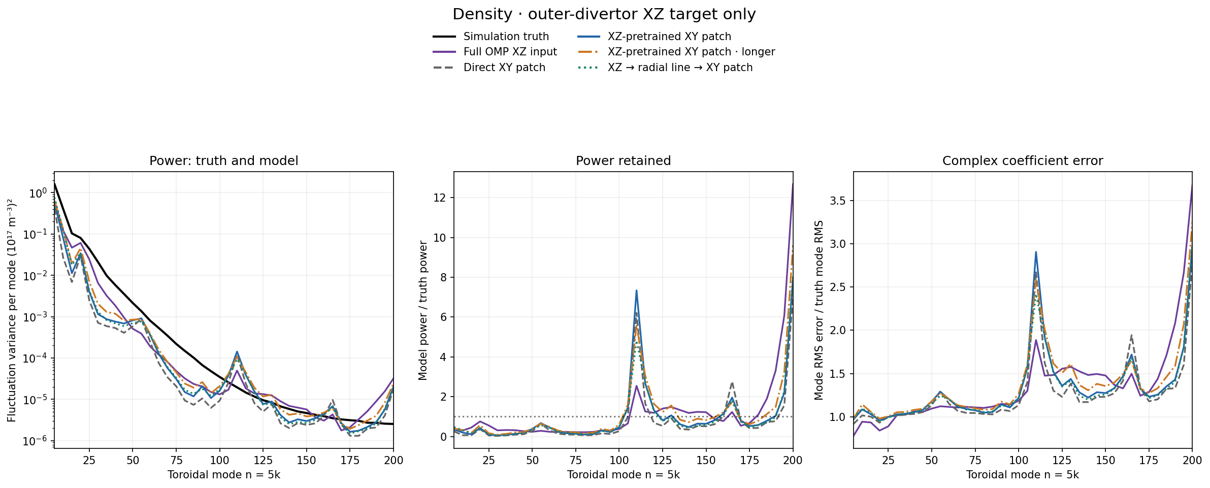
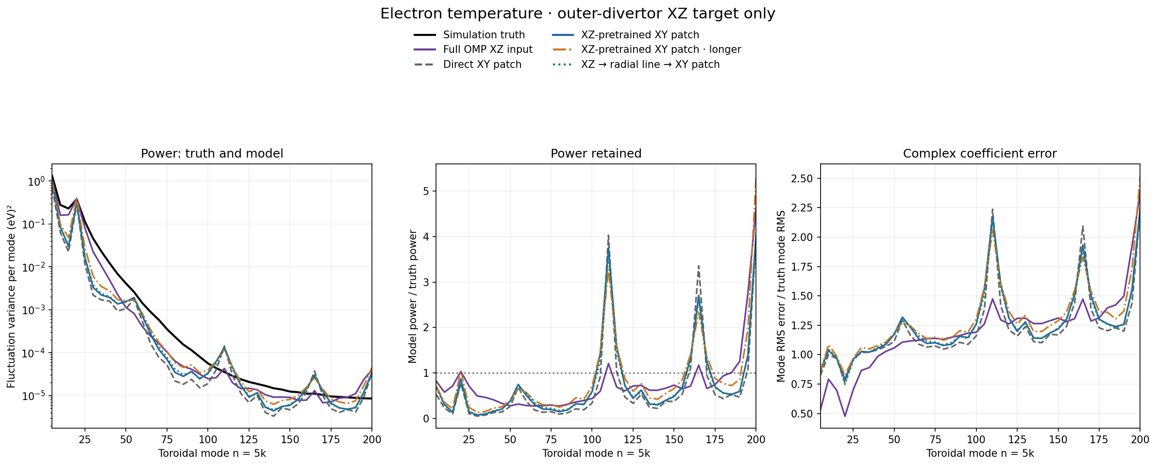
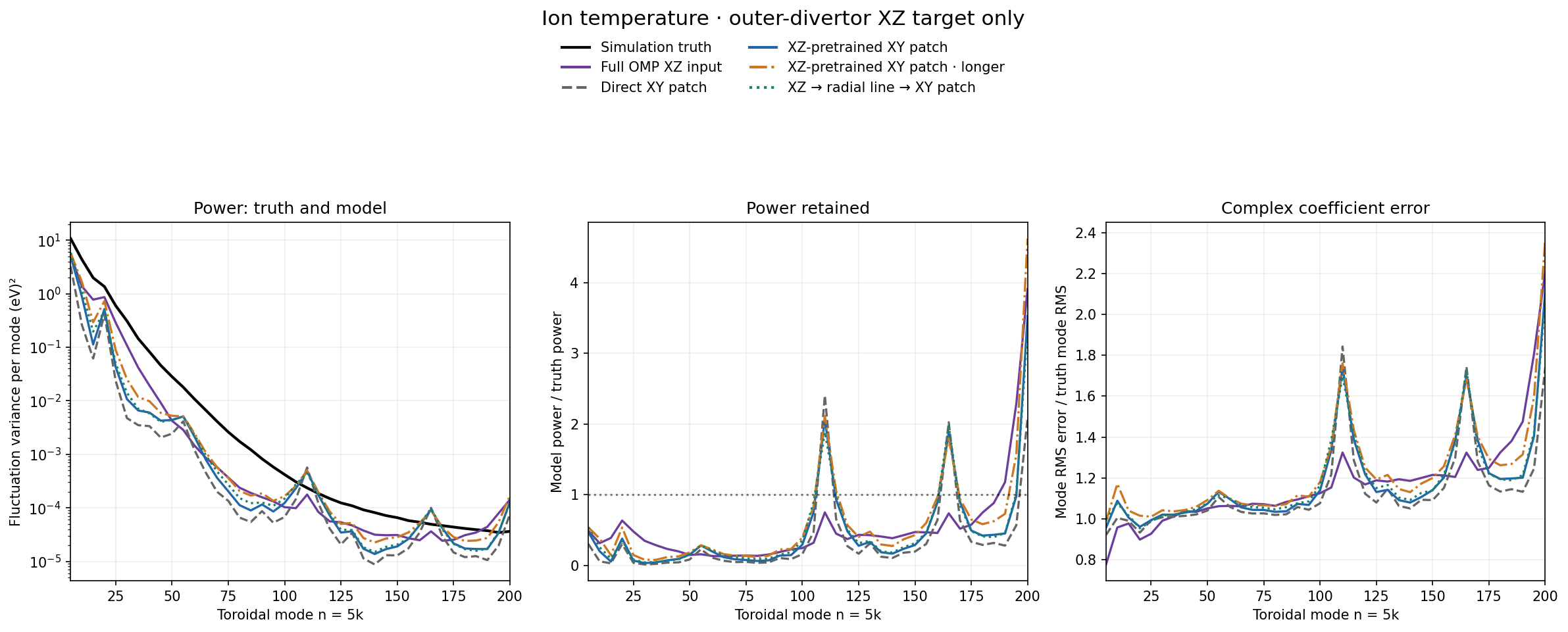
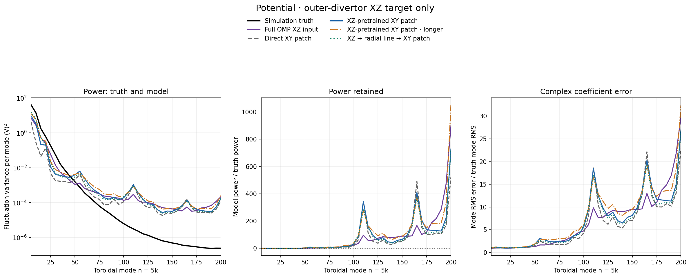
Same saved target-only evaluations as the earlier report. This is sparse-input inference at x16–63, y31, not full-volume reconstruction. Low-mode power is underestimated; sharp relative high-mode excess is amplified by very small truth power. The factor of two counts both ±k and changes truth and model together, not their ratio. The source of the narrow peaks is not yet established.
Outer-divertor power spectra · all five fields
Density target power and complex error. Exact target only. Left: nonzero-mode contribution to fluctuation variance (±k summed); middle: model/truth power; right: complex mode error divided by truth mode RMS. Averaged over the same124frames using native target-volume weights. Full n=5…200; no truncation. Download
Electron temperature target power and complex error. Exact target only. Left: nonzero-mode contribution to fluctuation variance (±k summed); middle: model/truth power; right: complex mode error divided by truth mode RMS. Averaged over the same124frames using native target-volume weights. Full n=5…200; no truncation. Download
Ion temperature target power and complex error. Exact target only. Left: nonzero-mode contribution to fluctuation variance (±k summed); middle: model/truth power; right: complex mode error divided by truth mode RMS. Averaged over the same124frames using native target-volume weights. Full n=5…200; no truncation. Download
Potential target power and complex error. Exact target only. Left: nonzero-mode contribution to fluctuation variance (±k summed); middle: model/truth power; right: complex mode error divided by truth mode RMS. Averaged over the same124frames using native target-volume weights. Full n=5…200; no truncation. Download
Parallel velocity target power and complex error. Exact target only. Left: nonzero-mode contribution to fluctuation variance (±k summed); middle: model/truth power; right: complex mode error divided by truth mode RMS. Averaged over the same124frames using native target-volume weights. Full n=5…200; no truncation. Download
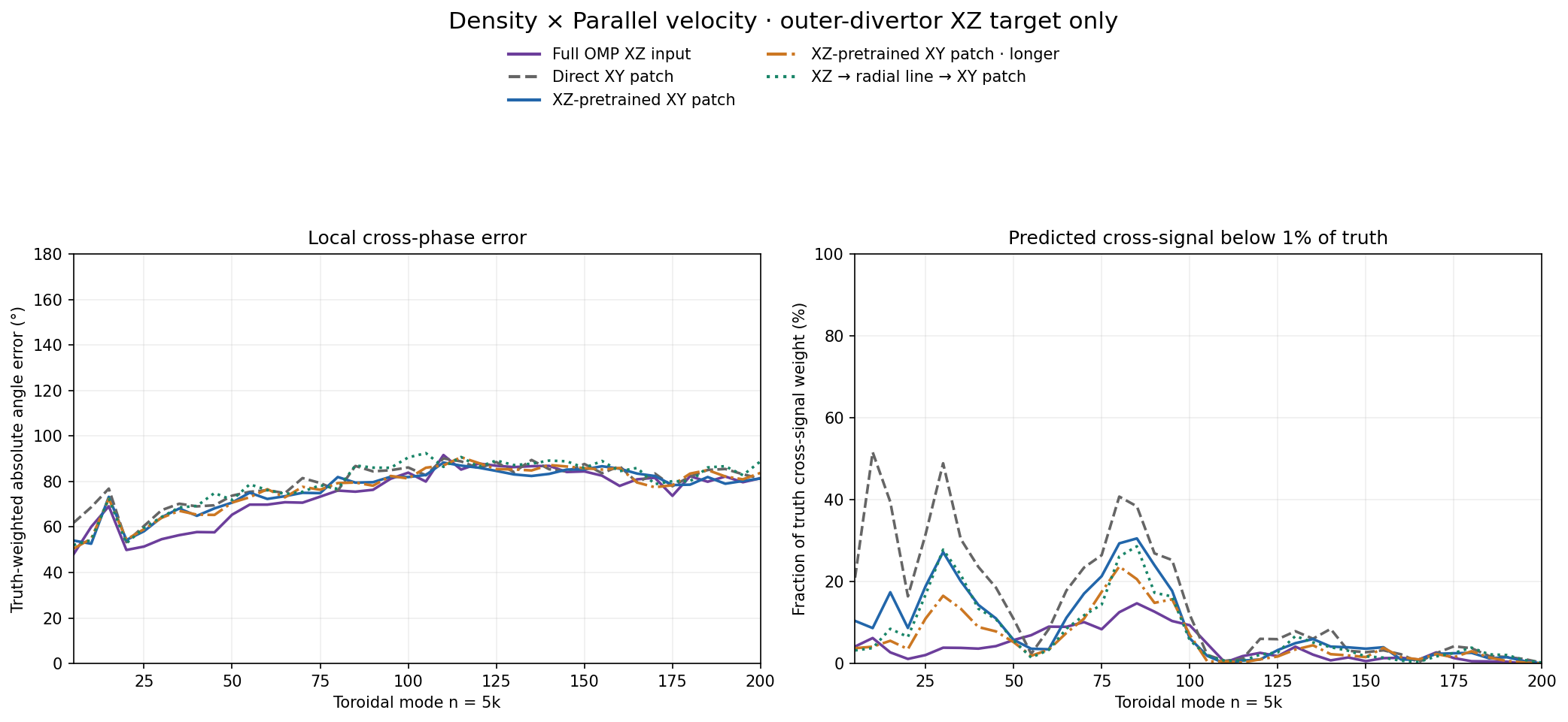
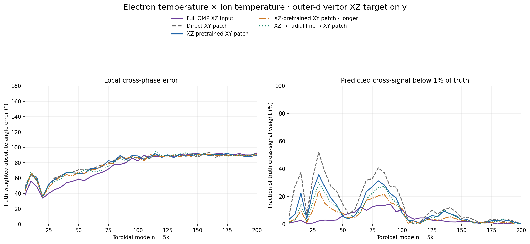
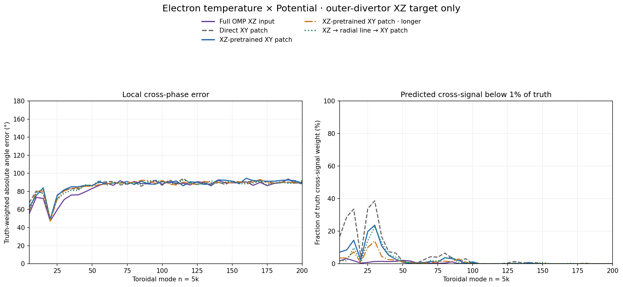
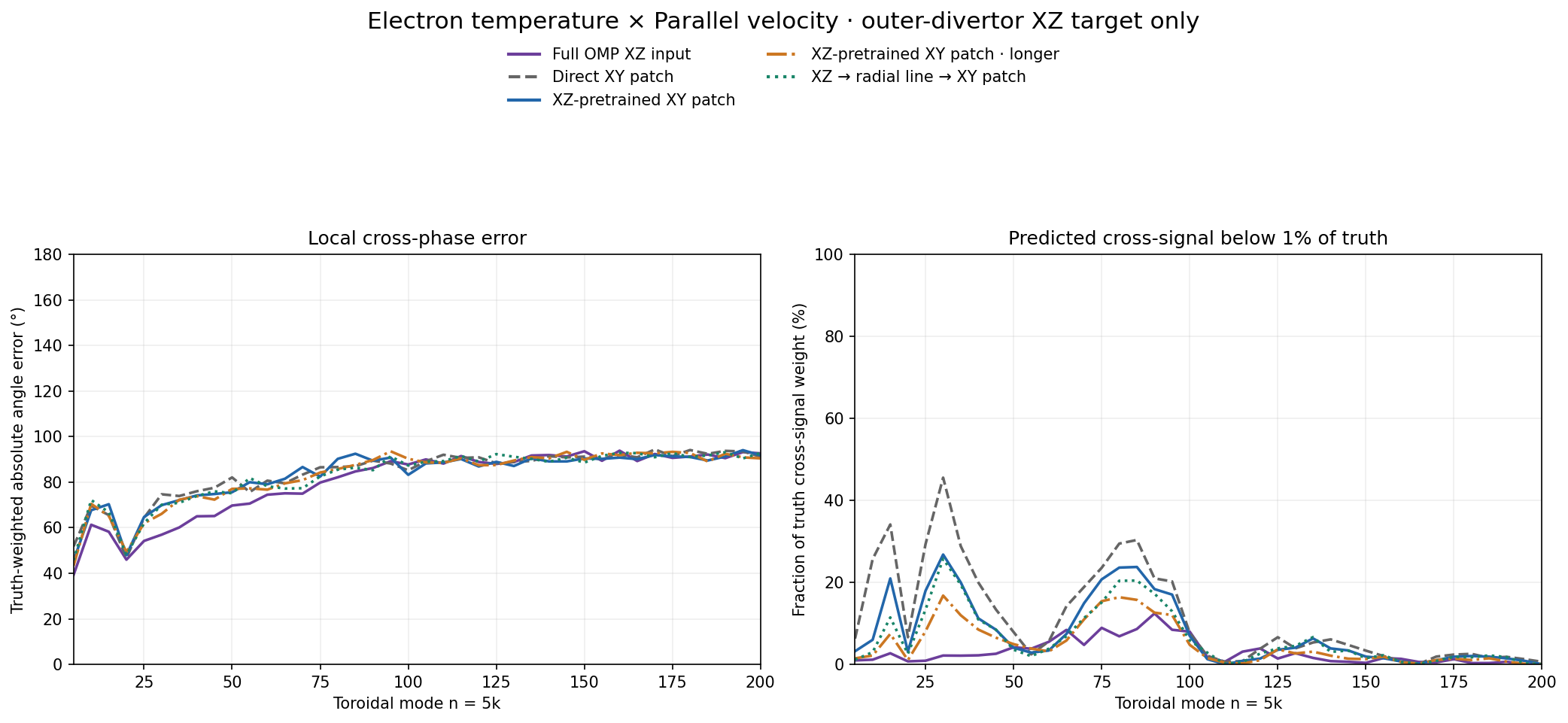
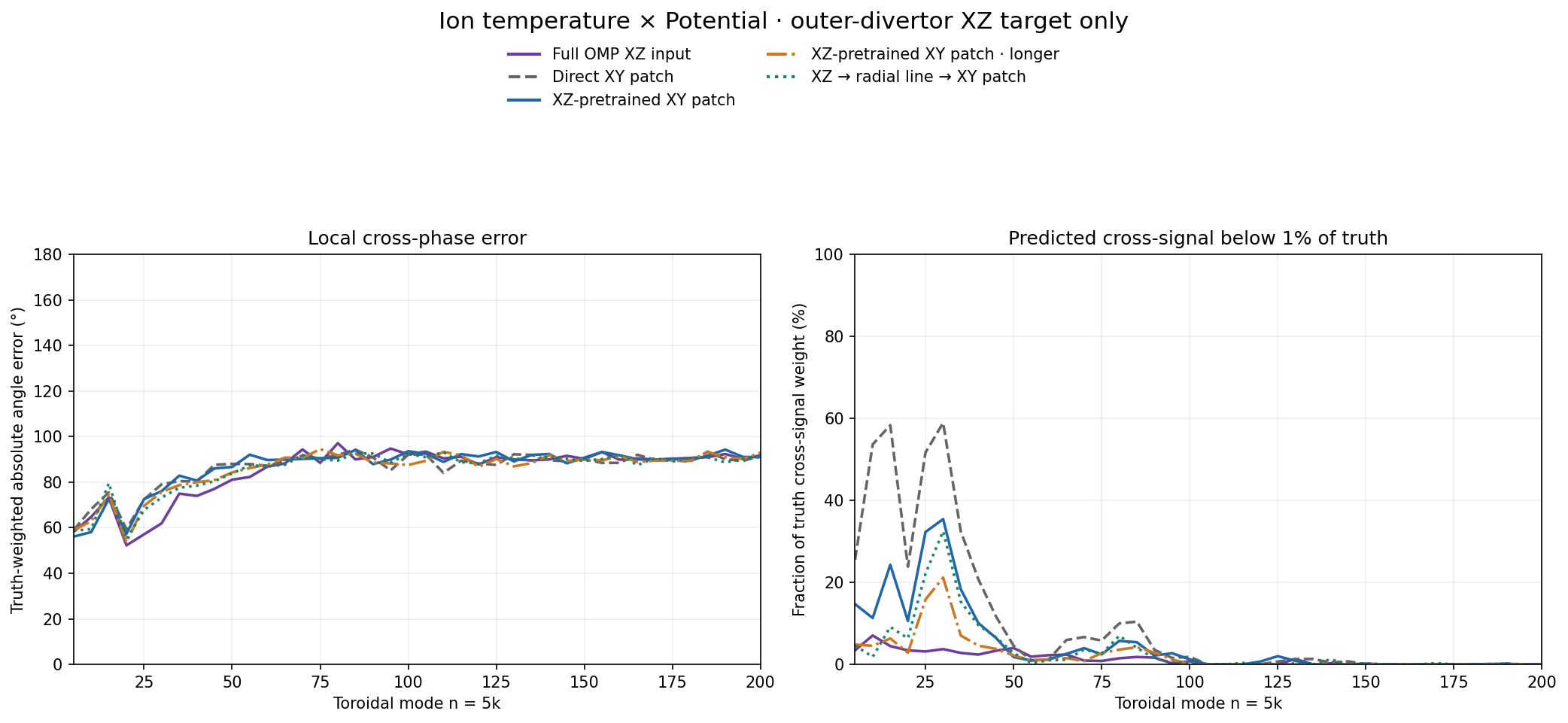
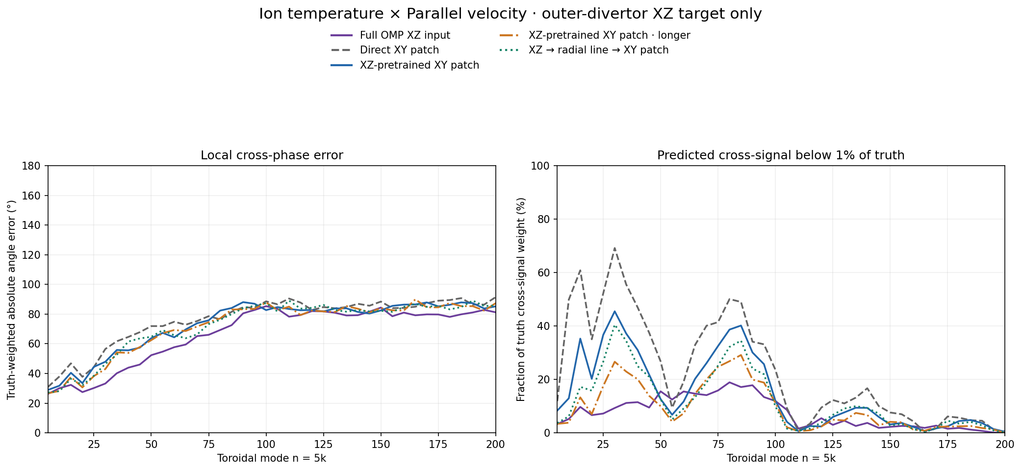
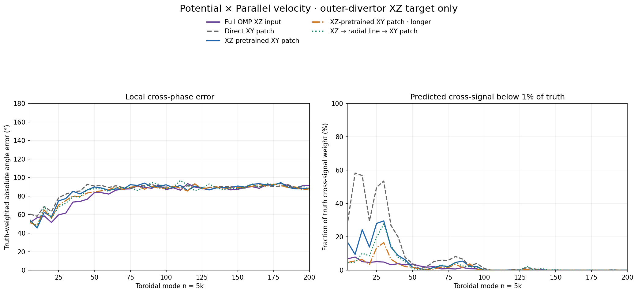
Outer-divertor LOCAL cross-phase error · all ten field pairs
Density × Electron temperature target local phase. Local model–truth wrapped-angle error is computed before averaging with native-volume × truth cross-amplitude weights. This is not pooled cross-phase. Saved estimator includes zero predicted amplitudes in its denominator, so read the adjacent below-1%-signal panel: a missing phase is not a valid accurate phase. Full n=5…200, same124validation frames. Download
Density × Ion temperature target local phase. Local model–truth wrapped-angle error is computed before averaging with native-volume × truth cross-amplitude weights. This is not pooled cross-phase. Saved estimator includes zero predicted amplitudes in its denominator, so read the adjacent below-1%-signal panel: a missing phase is not a valid accurate phase. Full n=5…200, same124validation frames. Download
Density × Potential target local phase. Local model–truth wrapped-angle error is computed before averaging with native-volume × truth cross-amplitude weights. This is not pooled cross-phase. Saved estimator includes zero predicted amplitudes in its denominator, so read the adjacent below-1%-signal panel: a missing phase is not a valid accurate phase. Full n=5…200, same124validation frames. Download
Density × Parallel velocity target local phase. Local model–truth wrapped-angle error is computed before averaging with native-volume × truth cross-amplitude weights. This is not pooled cross-phase. Saved estimator includes zero predicted amplitudes in its denominator, so read the adjacent below-1%-signal panel: a missing phase is not a valid accurate phase. Full n=5…200, same124validation frames. Download
Electron temperature × Ion temperature target local phase. Local model–truth wrapped-angle error is computed before averaging with native-volume × truth cross-amplitude weights. This is not pooled cross-phase. Saved estimator includes zero predicted amplitudes in its denominator, so read the adjacent below-1%-signal panel: a missing phase is not a valid accurate phase. Full n=5…200, same124validation frames. Download
Electron temperature × Potential target local phase. Local model–truth wrapped-angle error is computed before averaging with native-volume × truth cross-amplitude weights. This is not pooled cross-phase. Saved estimator includes zero predicted amplitudes in its denominator, so read the adjacent below-1%-signal panel: a missing phase is not a valid accurate phase. Full n=5…200, same124validation frames. Download
Electron temperature × Parallel velocity target local phase. Local model–truth wrapped-angle error is computed before averaging with native-volume × truth cross-amplitude weights. This is not pooled cross-phase. Saved estimator includes zero predicted amplitudes in its denominator, so read the adjacent below-1%-signal panel: a missing phase is not a valid accurate phase. Full n=5…200, same124validation frames. Download
Ion temperature × Potential target local phase. Local model–truth wrapped-angle error is computed before averaging with native-volume × truth cross-amplitude weights. This is not pooled cross-phase. Saved estimator includes zero predicted amplitudes in its denominator, so read the adjacent below-1%-signal panel: a missing phase is not a valid accurate phase. Full n=5…200, same124validation frames. Download
Ion temperature × Parallel velocity target local phase. Local model–truth wrapped-angle error is computed before averaging with native-volume × truth cross-amplitude weights. This is not pooled cross-phase. Saved estimator includes zero predicted amplitudes in its denominator, so read the adjacent below-1%-signal panel: a missing phase is not a valid accurate phase. Full n=5…200, same124validation frames. Download
Potential × Parallel velocity target local phase. Local model–truth wrapped-angle error is computed before averaging with native-volume × truth cross-amplitude weights. This is not pooled cross-phase. Saved estimator includes zero predicted amplitudes in its denominator, so read the adjacent below-1%-signal panel: a missing phase is not a valid accurate phase. Full n=5…200, same124validation frames. Download
Broader downstream region · separate from target-only plots
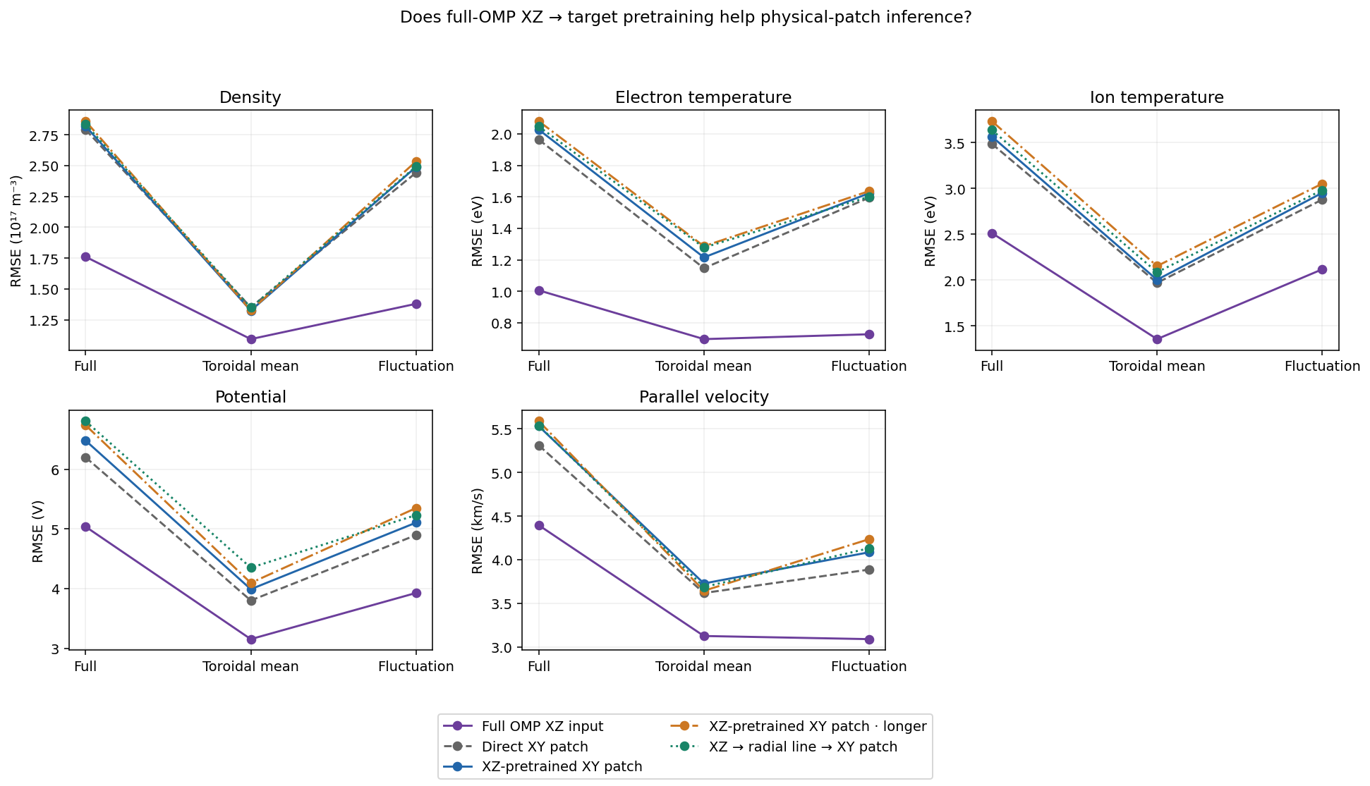
Downstream-volume full/mean/fluctuation errors. Same five models and fixed model key. These scores cover the broader downstream region; they are not the target-only errors above. Download
XZ-task pretraining did not make XY match XZ. On the exact target, the XZ-pretrained 30k patch model has about 20% higher density fluctuation error and 49% higher electron-temperature fluctuation error than full-XZ input. That gap is smaller than the 80%/123% increase in the broader downstream-volume scores. The direct-from-compressor patch model is better than the XZ-pretrained patch on all five exact-target fluctuation errors. The radial-line intermediate does not close the gap.
Which training stage and input do these labels mean?
Physical XY patch = nominal5×4cm R–Z window clipped to available radial coverage,64×21interpolated samples at one toroidal angle. Native radial line = all64radial cells at y18,z0. Full OMP XZ input = all64radial cells ×81toroidal samples at y18. Every model here predicts the outer-divertor XZ target. Five numerical fields, not GPI light. Curriculum configuration · Transport metrics, correlations and RMSE skill
Definitions used throughout
Term
Definition
Five fields
Ne: electron density (m⁻³); Te/Ti: electron/ion temperature (eV); phi: electrostatic potential (V); Vi: parallel ion velocity (m/s). Plot axes may rescale density or velocity.
Mean and fluctuations
q₀ is the instantaneous toroidal mean; q′=q−q₀. This is not subtraction of a fixed time average.
Ordinary physical MSE
Native-volume-weighted squared physical field error, normalized by fitting-only field variance.
Balanced objective
Equal normalized mean and fluctuation error contributions; each uses its fitting-only component scale with a standard-deviation floor.
GradNorm
Adaptive loss weights using gradient magnitudes/training rates; the patch objective learns component weights, not a new physical field.
RMSE / relative error
RMSE=sqrt(weighted mean squared error). Relative L2=RMS(error)/RMS(truth) on the stated support. Percentages are not percent of cells wrong.
RMSE skill
1−model RMSE / fitting-mean-baseline RMSE. Zero matches baseline; negative is worse. Saved correlations are accompanied by this skill.
Toroidal k and n
Fourier bin k; physical mode n=5k for the72° domain. n=0 is mean; resolved nonzero n=5…200.
Cross-phase
arg(q̂a · conjugate(q̂b)). Error is the wrapped model–truth angle difference. Local and pooled operations are not interchangeable.
Transport versus heat
Radial E×B particle/internal-energy transport and recovered divertor sheath heat are different operators on different spatial supports.
Clean replay
A full-input reconstruction loss added during sparse-observation adaptation; coefficient0.5 is not a50% example fraction.
Autoregression / diffusion
Autoregression feeds predictions back through time. Diffusion denoises a sampled target and can itself run autoregressively.
Full-target / residual
Full-target generates the future latent. Residual generates a correction to a deterministic forecast. Forecast conditioning alone does not make a residual model.